Using Recurrent Learning to Create Shakespeare Sonnets

Using an LSTM based Recurrent Learning model, we were able to quickly train the model to generate a new Shakespeare sonnet.

The thought of his but is the queen of the wind:
Thou hast done that with a wife of bate are to the
earth, and straker'd them secured of my own to with the
more.

CORIOLANUS:
My lord, so think'st thou to a play be with thee,
And mine with him to me, which think it be the gives
That see the componted heart of the more times,
And they in the farswer with the season
That thou art that thou hast a man as belied.

PRONEES:
That what so like the heart to the adficer to
the father doth and some part of our house of the server.

DOMIONA:
What wishes my servant words, and so dose strack,
here hores ip a lord.

PARELLO:
And you are grace; and a singer of your life,
And his heart mistress fare the dear be readors
To the buse of the father him to the sone.

HOMITIUS ENOBARY:
And they are not a his wonders for thy greater;
But but a plotering pastice and every sirs.

PAPOLLES:
I will not as my lord, and the prince and house,
But that is scort to my wanter with her than.

The thought of his but is the queen of the wind:

Thou hast done that with a wife of bate are to the

earth, and straker'd them secured of my own to with the

more.

CORIOLANUS:

My lord, so think'st thou to a play be with thee,

And mine with him to me, which think it be the gives

That see the componted heart of the more times,

And they in the farswer with the season

That thou art that thou hast a man as belied.

PRONEES:

That what so like the heart to the adficer to

the father doth and some part of our house of the server.

DOMIONA:

What wishes my servant words, and so dose strack,

here hores ip a lord.

PARELLO:

And you are grace; and a singer of your life,

And his heart mistress fare the dear be readors

To the buse of the father him to the sone.

HOMITIUS ENOBARY:

And they are not a his wonders for thy greater;

But but a plotering pastice and every sirs.

PAPOLLES:

I will not as my lord, and the prince and house,

But that is scort to my wanter with her than.

To create the Shakespeare above, we used the Char-RNN model shown below with the LSTM Layer.

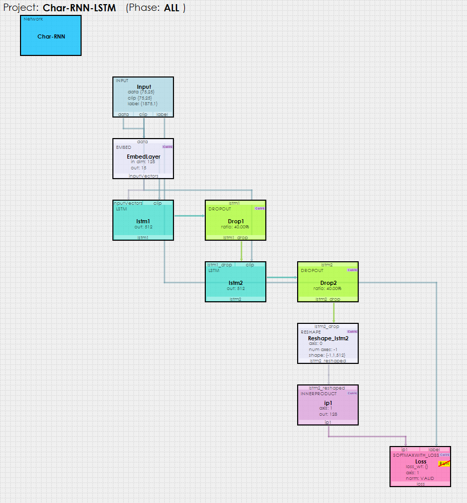
To solve this model, the SignalPop AI Designer uses the new MyCaffeTrainerRNN (which operates similarly to the MyCaffeTrainerRL) to train the recurrent network.

But what actually happens within each LSTM layer to make this happen?

Each LSTM layer contains an Unrolled Net which unrolls the recurrent operations. As shown below, you can see that each of the 75 elements within the sequence are ‘unrolled’ into a set of layers: SCALE, INNER_PRODUCT, RESHAPE and LSTM_UNIT. Each set process the data and feeds it into the next thus forming the recurrent nature of the network.

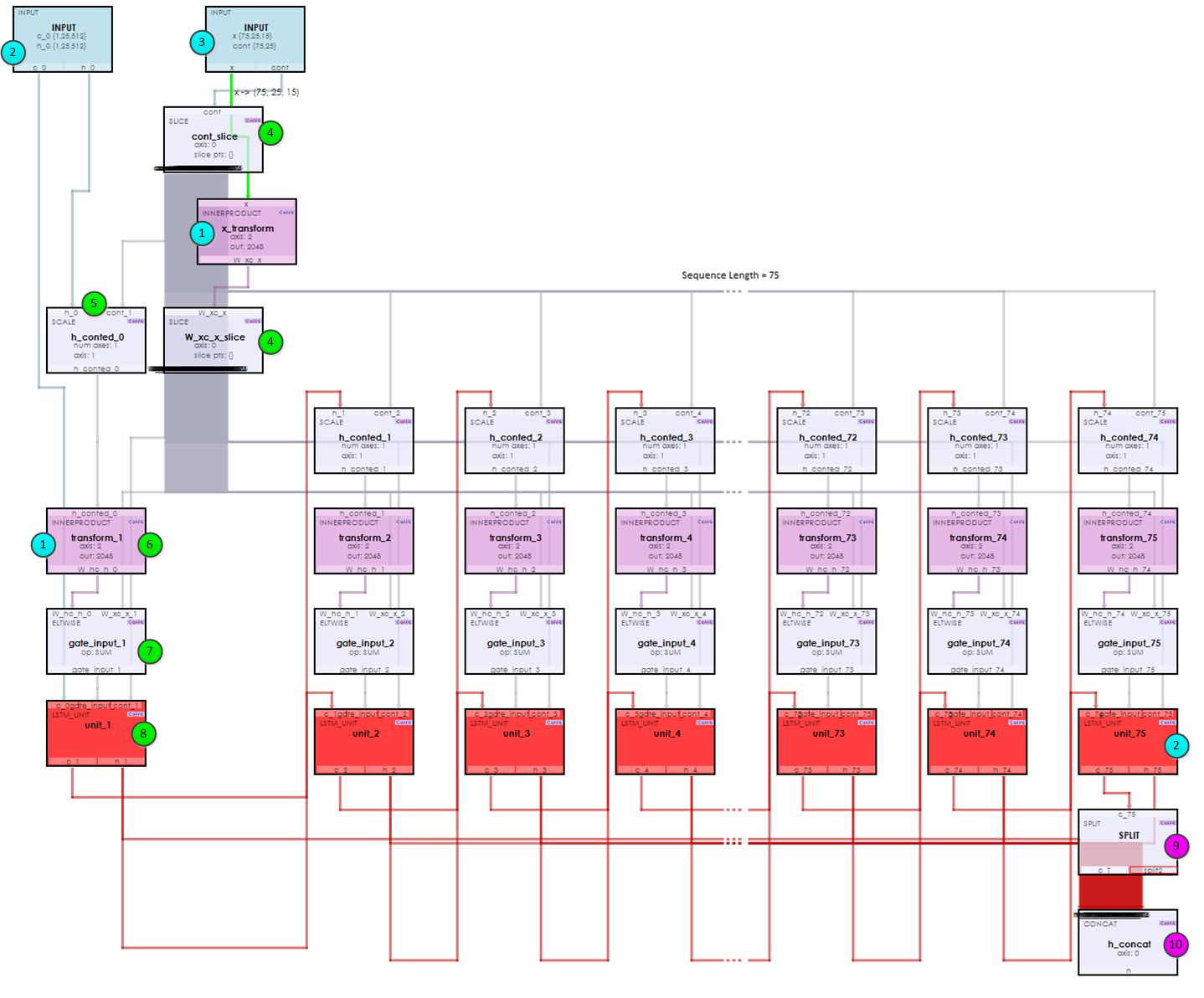
During the initialization (steps 1-3) the weights are loaded and data is fed into the x input blob. Next in steps 4-8, the recurrent nature of the network processes the each item within the sequence. Upon reaching the end the results are concatenated to form the output in steps 9 and 10. This same process occurs in both LSTM layers – so the full Char-RNN actually has over 600 layers. Amazingly all of this processing for both the forward and backward pass happens in around 64 milliseconds on a Titan Xp running in TCC mode!

To try out this model and train it yourself, just check out our Tutorials for easy step-by-step instructions that will get you started quickly! For cool example videos, including a Cart-Pole balancing video, check out our Examples page.