

This tutorial will guide you through the steps to create and train a Temporal Fusion Transformer, based on [1] and [2] to predict electrical usage.
Note: with a batch size of 64, this tutorial requires 6.5 GB of GPU memory. If you do not have this much GPU memory, reduce the batch size in each of the three DataTemporal layers.
Step 1 – Download the Raw Data
In the first step, you must download the raw data using the MyCaffe Test Application which is located in the MyCaffe Test Application Releases. The raw data contains the UCI Electricity Load Diagrams Dataset.
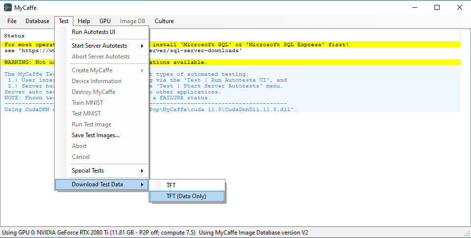
Once installed, select the ‘Test | Download Test Data | TFT (Data Only)’ menu item and select the Run button from the Test Data Download dialog.
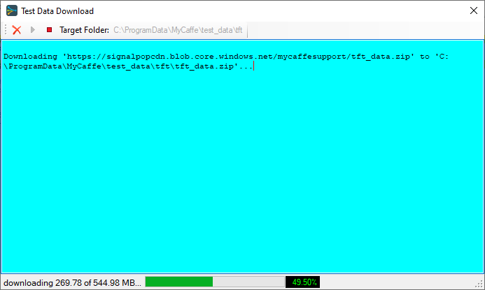
After the download completes, the raw data file LD2011_2014.txt will be placed in the following directory:
C:\ProgramData\MyCaffe\test_data\tft\data\electricity
Step 2 – Pre-Process the Raw Data
The SignalPop AI Designer TFT_electricity Dataset Creator is used to pre-process the data by aggregating to hourly time periods, normalizing, and organizing the data into a train, test, and validation data-set suitable for the TFT model.
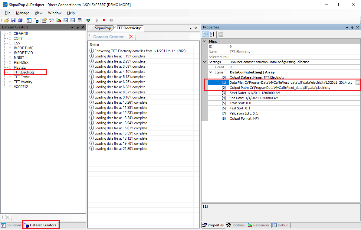
From the lower left corner of the SignalPop AI Designer, select the Dataset Creators tab and double click on the TFT_electricity Dataset Creator to display its status and properties window.
Enter the following properties and select the Run ((![]() ) button to start pre-processing the data:
) button to start pre-processing the data:
Data File:
C:\ProgramData\MyCaffe\test_data\tft\data\electricity\LD2011_2014.txt
Output Path:
C:\ProgramData\MyCaffe\test_data\tft\data\electricity
The preprocessed data will be placed into the following directory.
C:\ProgramData\MyCaffe\test_data\tft\data\electricity\preprocessed
Step 3 – Create the Temporal Fusion Transformer Model
Next, we need to create the TFT_electricity project that uses the MODEL (temporal) based dataset. MODEL (temporal) based datasets rely on the model itself to collect the data used for training.
First select the Add Project ((![]() ) button at the bottom of the Solutions window, which will display the New Project dialog.
) button at the bottom of the Solutions window, which will display the New Project dialog.
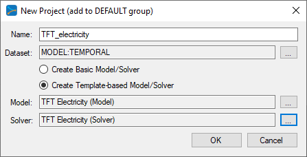
To select the MODEL (temporal) dataset, click on the ‘…’ button to the right of the Dataset field and select the MODEL (temporal) radio button at the bottom of the dialog.
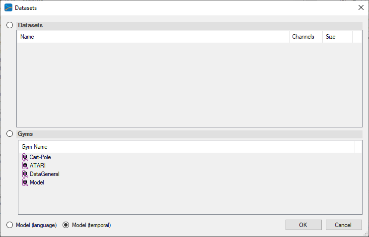
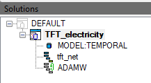
Upon selecting OK on the New Project dialog, the new TFT_electricity project will be displayed in the Solutions window.
Step 4 – Review the Model
Double click on the tft_net model name within the TFT_electricity project to display the model editor, allowing you to revie the model. As you can see below, the TFT models are quite complex.
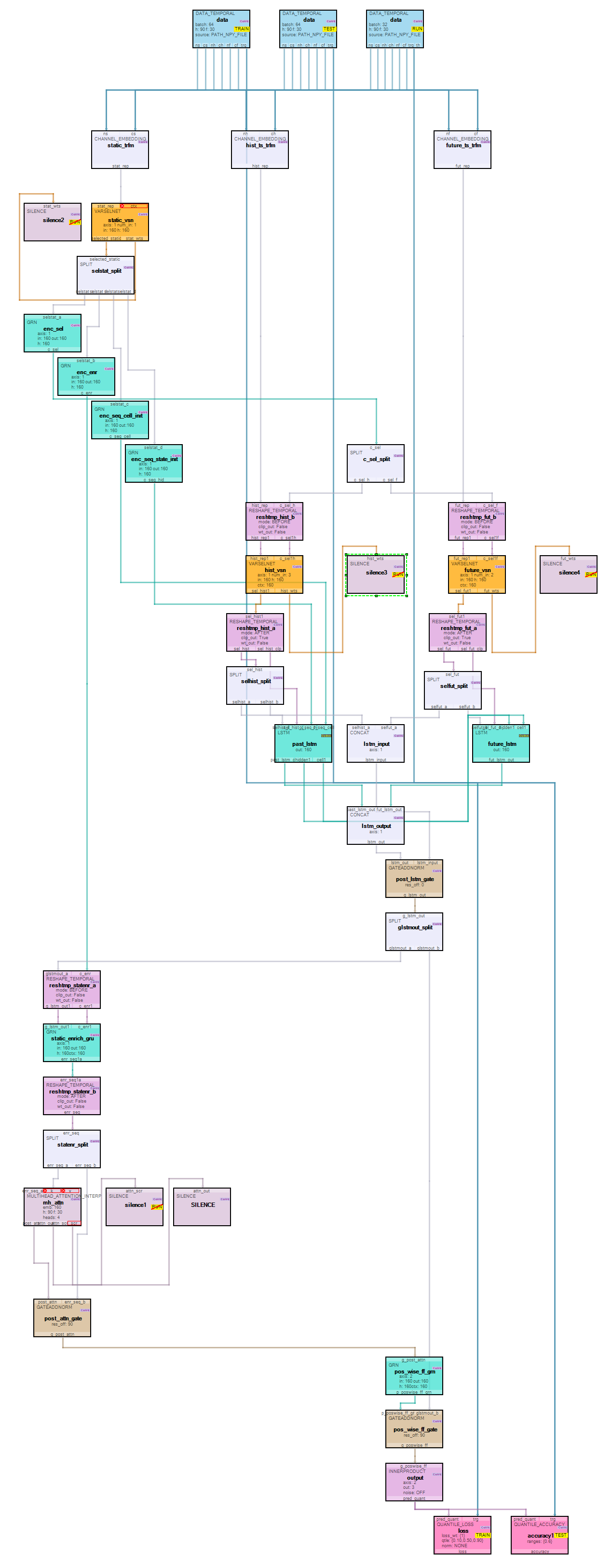
The TFT model used to predict electricity usage uses 90 historical steps and predicts 30 future steps. For data inputs, the model takes 1 static input (customer id), 3 historical inputs (log power usage, hour, and hours from start) and 2 future inputs (hour and hours from start). Quantiles are predicted over the 30 future steps for 10, 50 and 90.
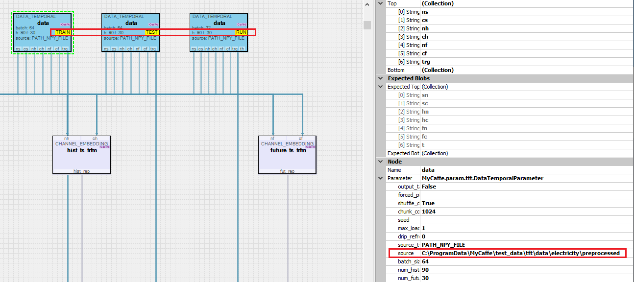
Note, the source property of each Data Temporal layer points to the output directory where all pre-processed data is placed by TFT_electricity Dataset Creator. The pre-processed data is loaded based on its type and the specific phase of the Data Temporal layer. For example, the Data Temporal layer with the ‘TRAIN’ phase (on the left above) loads the following pre-processed data:
train_known_num.npy
train_observed_num.npy
train_schema.xml
train_static_cat.npy
train_sync.npy
Step 5 – Training
The training step uses the ADAMW solver but with no weight decay (the ADAM may be used as well) and a base learning rate of 0.001, momentum = 0.9 and momentum2 = 0.999.
We trained on an NVIDIA 2080 Ti with a batch size of 64; historical steps = 90 and future steps = 30. With these settings, the model uses 7.68GB of the 2080 TI’s 11.8GB of GPU memory.
To start training, first open the project by right clicking on the TFT_electric project and selecting the ‘Open’ menu option. Next, double click on the TFT_electric project name to open the project window and select the Run Training ((![]() ) button.
) button.
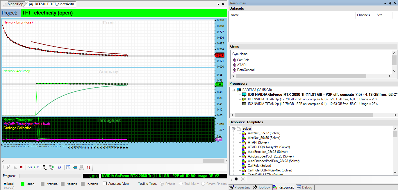
We trained the model for around 1000 iterations.
Step 6 – Analyze the Results
After training for around 1000 iterations or so, stop the training, check the ‘Test Many’ radio button at the bottom middle of the Project window. Next, select the Run Testing ((![]() ) button which will then display the Test Many dialog.
) button which will then display the Test Many dialog.
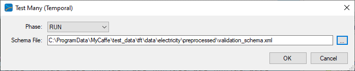
Select the validation_schema.xml file from the preprocessed directory for the electricity data. This file contains the data layout used to determine which variables are associated with the weights withing the VSN layers.
After pressing OK, the analytics are displayed showing several predictions and how they match up with the target data.
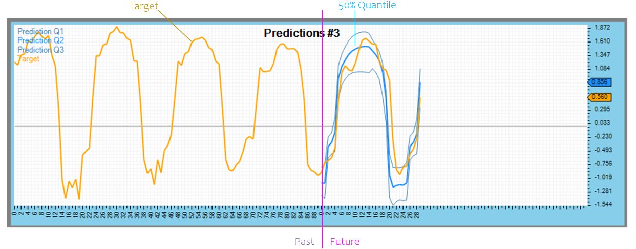
Predicted quantiles are shown in blue for the future portion only, whereas the target data is shown in orange.
After the prediction data you will find the variable analysis from each of the three Variable Selection Networks. The variable analysis is shown on a per variable basis and then on a temporal basis.
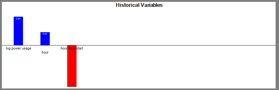
The per variable basis shows which variables contributed most to the predicted results. For example, the ‘log power usage’ variable contributed most in the historical variables to the results.
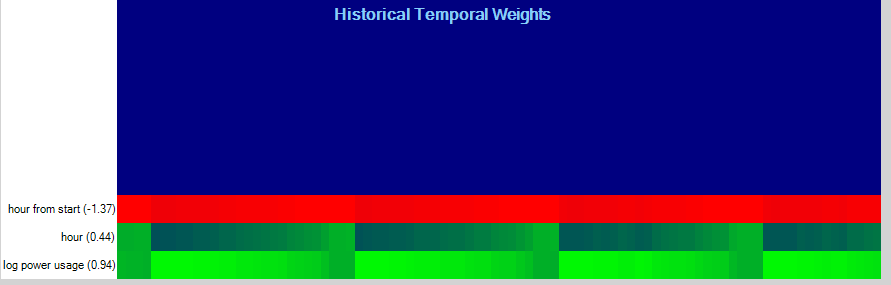
The temporal variable analysis looks at the temporal weightings for each variable observed on a randomly selected input. This analysis can show a periodicity in the data.
And finally, the attention scores are analyzed across multi-percentiles and multi-horizons.
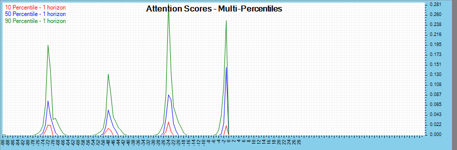
The image above shows the percentiles for each of the three quantiles used (10, 50 and 90) which all show a strong periodic behavior with a 24-hour cycle.
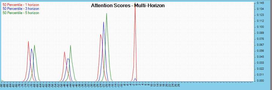
The multi-horizon attention scores are viewed across time horizons with the 50-percentile data.
Note on Using SQL Data Source for Electricity TFT
The sample above uses the NPY files created by the SignalPop AI Designer TFT.Electricity dataset creator. This dataset creator can also load all electricity data into a SQL database.
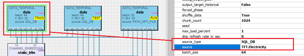
Using the SQL database data source instead of the Numpy file can be accomplished with the following steps:
- Open the TFT_electricity project model as described in Step 4 above.
- Select each of the data layers and change the source_type to SQL_DB and source to TFT.Electricity.
- Save the project, and train the project and data will now be loaded from the SQL databased instead of the NPY files.
Congratulations! You have now created and trained your first TFT model using MyCaffe!
[1] Bryan Lim, Sercan O. Arik, Nicolas Loeff, and Tomas Pfister, Temporal Fusion Transformers for Interpretable Multi-horizon Time Series Prediction, 2019, arXiv:1912.09360.
[2] GitHub: PlaytikaOSS/tft-torch, by Playtika Research, 2021, GitHub