

This tutorial will guide you through the steps to create an Auto-Encoder model and train it on the MNIST dataset as described by [1].
Step 1 – Create the Dataset
Before creating the Auto-Encoder model, you will need to download the MNIST data files from here and create the single channel MNIST dataset.
To create the dataset, open the MNIST Dataset Creator from the Dataset Creators pane and add the file locations of each of the MNIST data files downloaded above. Next, make sure the Channels property is set to 1 and select the Run (![]() ) button to start creating the dataset.
) button to start creating the dataset.
To view the new MNIST dataset, expand the MNIST Dataset Creator and double click on the new MNIST dataset.
Double clicking on any image will show a larger view of the image and right clicking in an area other than an image displays a menu that allows you to view the Image Mean.
Once completed, the new dataset will be named MNIST and look as follows.
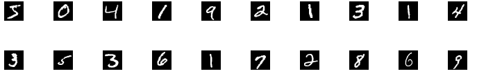
The MNIST dataset contains 60,000 training and 10,000 testing images of hand written digits.
Step 2 – Creating the AUTO-ENCODER Model
The first step in creating a model is to select Solutions pane and then press the Add Project (![]() ) button at the bottom pane.
) button at the bottom pane.
Next, fill out the New Project dialog with the project name, MNIST dataset, select Create Template-based Model/Solver and use the AutoEncoderPool_28x28 model and AutoEncoderPool_28x28 solver templates. Note, to create the non-pooled version, use the AutoEncoder_28x28 templates.
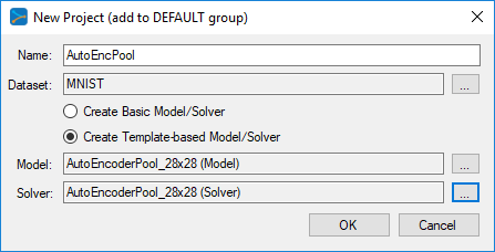
After pressing OK, the new AutoEncPool project will be added to the solutions.
To view the Auto-Encoder model, just double click on the AutoEncPoolNet item within the AutoEncPool project. This will open the visual model editor containing the deep convolutional auto-encoder (with pooling) model which looks as follows.
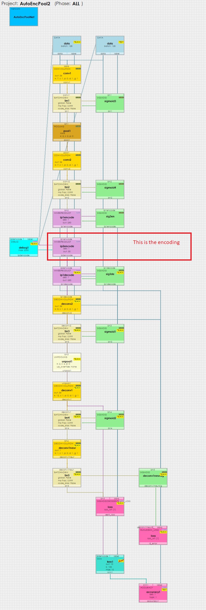
At the center of the model you will notice the ip2encode layer – this layer holds the 30 item encoding that the model learns by learning to re-generate the inputs with all layers that follow.
You are now ready to train the model.
Step 3 – Training the Auto-Encoder Model
When training, we recommend using a TCC enabled GPU such as the NVIDIA Titan Xp. To enable TCC mode, see the documentation for nvidia-smi paying special attention to the -g and -dm commands. For example the following command will set GPU 0 into the TCC mode.
nvidia-smi -g 0 -dm 1
IMPORTANT: When using TCC mode in a multi-GPU system, we highly recommend setting all headless GPU’s to use the TCC mode for we have experienced stability issues when mixing headless GPU’s between the WDM and TCC modes.
NOTE: Using a TCC enabled GPU is not required, but training can be substantially faster than when training in WDM mode.
To start training, press the Run Training (![]() ) button in the lower left corner of the Project Window.
) button in the lower left corner of the Project Window.
After training for around 2000 iterations with a batch size of 128, you should see an accuracy of 74% or greater.
Step 4 – Inspecting Your Model
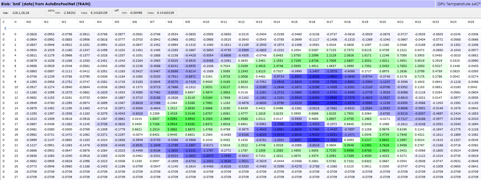
Once training completes, you can view the images produced by the network by right clicking on the last BATCHNORM layer named bn5 and selecting the Inspect Layer menu item (Note, make sure the network is in the open state when you do this).
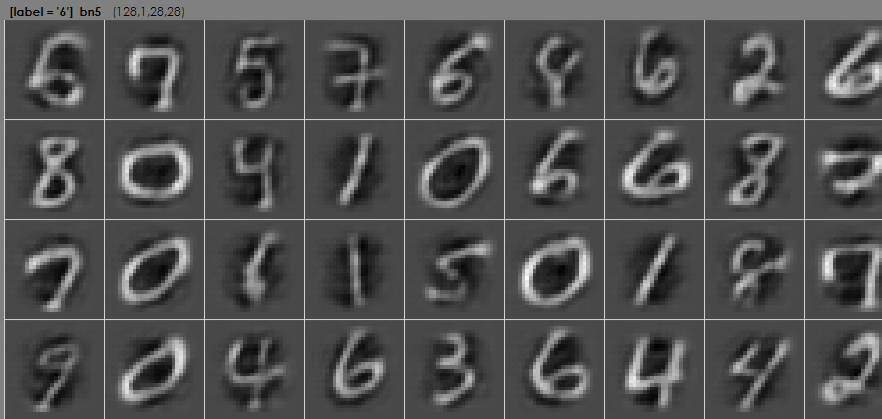
Inspecting a layer, shows the visual representation of the data within that layer, and in the case of the bn5 layer shows the output of the learned data of the network. As you can see above, the network has learned to produce the inputs.
Blob Data Window
To view the actual value of the first image of the output, select the Inspect Single Items (![]() ) button in the lower part of the model editor. Next, select the link between the bn5 and loss layer turning the link bright green. Right click on the selected link and select the Inspect Link Data menu item to display the data flowing through the link in the Blob Data window.
) button in the lower part of the model editor. Next, select the link between the bn5 and loss layer turning the link bright green. Right click on the selected link and select the Inspect Link Data menu item to display the data flowing through the link in the Blob Data window.
Embedding Data Separation
After confirming that your model is actually learning how to produce the inputs, the next step is to see how well the model has learned to separate the different classes of inputs.
To analyze this information you will need to inspect the DEBUG layer.
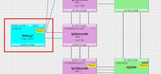
The DEBUG layer acts as a pass-through in that all data sent to it is cached and then passed on through. Inspecting this layer runs the t-SNE algorithm on the cached data so that you can actually see the data separation. An example of this is shown below.
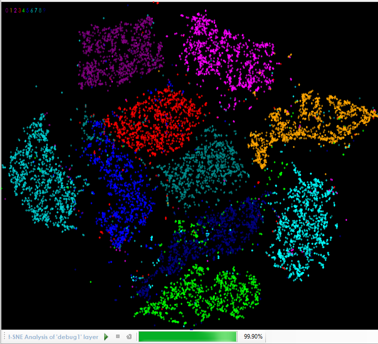
The t-SNE analysis of the Auto-Encoder shows a clear separation of the classes within the encoding.
You have now created your first Auto-Encoder for the MNIST dataset using the SignalPop AI Designer!
Step 5 – Using Auto-Encoder as Pre-Training
Now that you have trained your auto-encoder, it is time to use it to pre-train your actual classification model.
First, you will need to export the weights of your trained Auto-Encoder model. The weights are exported by right clicking the Accuracy sub-tree item of the AutoEncPool project and selecting the Export | Weights menu item.
Next, you will need to create the classification model by following step 2 above, but with the AutoEncoderPoolRun_28x28 model and solver templates. This will create a new model just up to the embedding with a standard classification ending set of layers.
And finally, you will need to import the weights of the AutoEncPool project into your new AutoEncPoolRun project. To do this, open the AutoEncPoolRun project by right clicking on the project and selecting the Open menu item. Once open, right click on its Accuracy sub-tree item and select the Import menu item which will display the dialog below when loading the previously exported weight file.
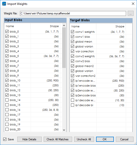
The importing process automatically selects all matching blobs. Select the Save check box and press OK to import the weights.
Once imported, you are ready to perform the final training of the new project which can be accomplished by opening the project pressing the Run Training button (![]() ) in the lower left corner of the Project Window.
) in the lower left corner of the Project Window.
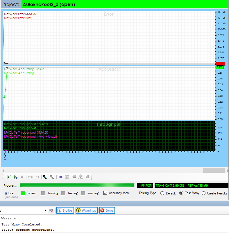
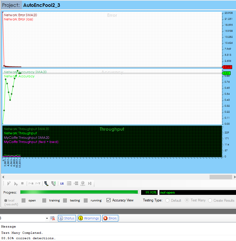
Comparing Pre-Training to Standard Training
The following model was trained with pre-training up to 97% accuracy within 3000 iterations.
The same model was trained to around 92%+ accuracy after 10,000 iterations when using regular training.
Clearly the pre-training helped accelerate the training of the model which is why the technique of using Auto-Encoders for pre-training has gained popularity.
[1] Volodymyr Turchenko, Eric Chalmers, Artur Luczak, A Deep Convolutional Auto-Encoder with Pooling – Unpooling Layers in Caffe. arXiv, 2017.