

This tutorial will guide you through the steps to create a Sigmoid based Policy Gradient Reinforcement Learning model as described by Andrej Karpathy [1][2][3] and train it on the Cart-Pole gym inspired by OpenAI [4][5] and originally implemented by Richard Sutton et al. [6][7].
Step 1 – Create the Project
In the first step we need to create a new project that contains the Cart-Pole gym, the simple Policy Gradient model and the RMSProp solver.
To do this, first select the Add Project (![]() ) button at the bottom of the Solutions window, which will display the New Project dialog.
) button at the bottom of the Solutions window, which will display the New Project dialog.
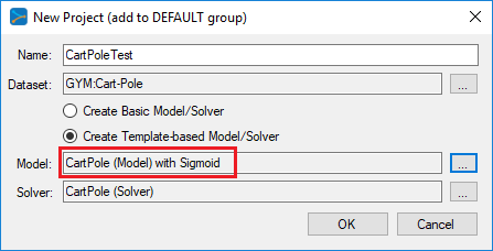
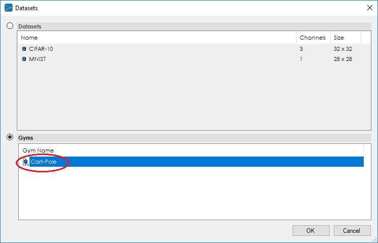
To add the Cart-Pole gym, press the Browse (…) button to the right of the Dataset: field which will display the Datasets dialog.
Next, add the Cart-Pole model and solver using the Browse (…) button next to the Model: and Solver: fields.
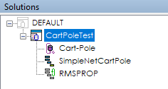
Upon selecting OK on the New Project dialog, the new CartPoleTest project will be displayed in the Solutions window.
Step 2 – Review the Model
Now that you have created the project, lets open up the model to see how it is organized. To review the model, double click on the SimpleNetCartPole model within the new CartPoleTest project, which will open up the Model Editor window.
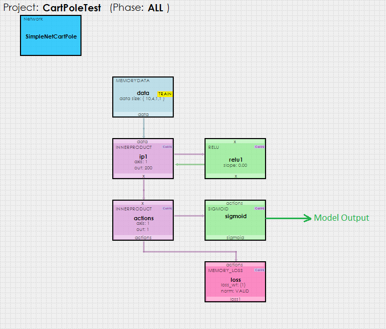
As you can see, the policy gradient reinforcement learning model used is fairly simple, comprising of just two inner product layers.
A MemoryData layer feeds batches of 10 items, each with 4 data values received on each step of the Cart-Pole simulation. The 4 data values used on each step are:
1.) x position
2.) x acceleration
3.) pole angle (in radians)
4.) pole acceleration (in radians)
A difference is created between the current step and the previous step, which is then fed into the MemoryData layer and proceeds on down the model during the forward pass.
The Sigmoid layer provides the network output which is treated as a probability that is used to determine whether or not to move the cart to the left or right.
The MemoryLoss layer calculates the loss and gradients which are then fed back up through the network during the backward pass.
Training Process
The new MyCaffeTrainerRL performs the training, during which data is received from the Cart-Pole gym at each step that the simulation runs. The gym runs until the cart either runs off the track to the right or left, or until the pole angle exceeds +/- 20 degrees. A single run comprises a set of steps that as a group are called an episode. During each run, steps 1-4 (image below) take place:
1.) First a state difference (current state – previous state) is fed through the model causing the Sigmoid layer to produce the output, which is treated as a probability that tells us which action to take – this probability is called Aprob.
2.) Next, the Aprob is converted into an Action (if a random number is < Aprob, go left, otherwise go right). The action is used to run the next step in the simulation, which also gives us the reward for taking that action.
3.) The initial gradient is calculated as a value that “encourages the action that was taken, to be taken.” [2][3] Aprob is the probability of what action the network ‘thinks’ should be taken, where as the Action is the actual action taken.
4.) Next, the state, action taken on the state, the rewards from taking the action, and the initial gradient Dlogps are batched up until the episode ends.

Upon the completion of the episode, the training begins by calculating the Policy Gradients and pushing them on up through the network with a Solver step, where the solver is instructed to accumulate the gradients. During this process, the following steps occur:
5.) First the discounted rewards are calculated back in time so as to emphasize the more near-term rewards.
6.) Next, the original policy gradient is modulated by multiplying it (Dlogps) by the discounted rewards. NOTE: A Dlogps value exists for each step in the batch as does a discounted reward, so the final policy gradient contains a gradient for each step, where each is modulated by the discounted reward for the step. “This is where the policy gradient magic occurs.”[2].
7.) The policy gradient is then copied to the bottom diff for the ‘actions‘ InnerProduct layer connected to the MemoryLoss layer…
8.) … which is then back-propagated back up through the network.
Solver Settings
The RMSProp solver is used to solve the policy gradient RL model with the following settings.
Learning Rate (base_lr) = 0.001
Weight Decay (weight_decay) = 0
RMS Decay (rms_decay) = 0.99
The MyCaffeTrainerRL that trains the open MyCaffe project uses the following specific settings.
Trainer Type = PG.MT; use the policy gradient trainer.
Reward Type = VAL; specifies to output the actual reward value. Other settings include MAX which only outputs the maximum reward observed.
Gamma = 0.99; specifies the discounting factor for discounted rewards.
Init1 = 10; specifies to use a force of +/- 10 to move the cart.
Init2 = 0; specifies to use non-additive forces. When 1, the current force is added to the previous force already used.
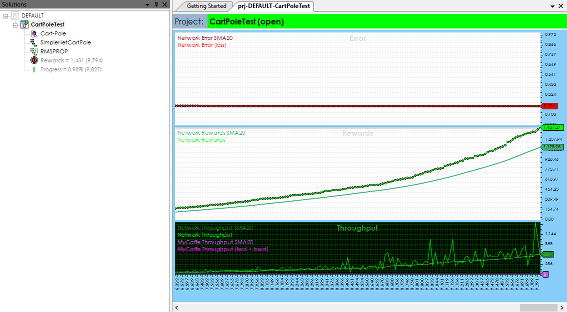
Step 3 – Training
Now that you are all set up, you are ready to start training the model. Double click on the CartPoleTest project to open its Project window. To start training, select the Run Training (![]() ) button in the bottom left corner of the Project window.
) button in the bottom left corner of the Project window.
To view the Cart-Pole gym simulation while the training is taking place, just double click on the Cart-Pole (![]() ) gym within the CartPoleTest project. This will open the Test Gym window that shows the running simulation.
) gym within the CartPoleTest project. This will open the Test Gym window that shows the running simulation.
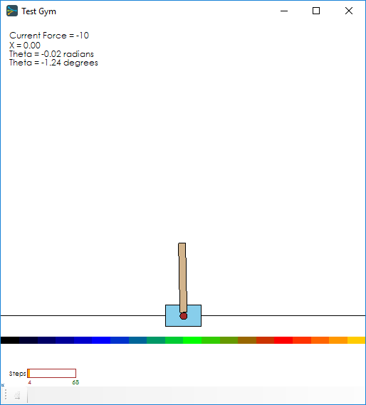
IMPORTANT: When open, the training will slow down to account for the 30 frames-per-second timing used to display the simulation. To speed up training, merely close the window.
Congratulations! You have now built your first policy gradient reinforcement learning model with MyCaffe and trained it on the Cart-Pole gym!
The video below shows the policy gradient model in action, balancing the pole for over a minute.
To see the SignalPop AI Designer in action with other models, see the Examples page.
[1] Karpathy, A., Deep Reinforcement Learning: Pong from Pixels, Andrej Karpathy blog, May 31, 2016.
[2] Karpathy, A., GitHub:karpathy/pg-pong.py, GitHub, 2016.
[3] Karpathy, A., CS231n Convolutional Neural Networks for Visual Recognition, Stanford University.
[4] OpenAI, CartPole-V0.
[5] OpenAI, GitHub:gym/gym/envs/classic_control/cartpole.py, GitHub, April 27, 2016.
[6] Barto, A. G., Sutton, R. S., Anderson, C. W., Neuronlike adaptive elements that can solve difficult learning control problems, IEEE, Vols. SMC-13, no. 5, pp. 834-846, September 1983.
[7] Sutton, R. S., et al., incompleteideas.net/sutton/book/code/pole.c, 1983.