Closed-form Continuous-time Liquid Neural Net Models

Liquid neural networks, first introduced by [1], are networks constructed “of linear first-order dynamical systems modulated via nonlinear interlinked gates,” resulting in models that “represent dynamical systems with varying (i.e., liquid) time-constants coupled to their hidden state, with outputs being computed by numerical differential equation solvers.”

The Closed-form Continuous-time Models (CfC) ‘are powerful sequential liquid neural processing units.” [2] CfC models “closely approximate liquid time-constant networks (LTCs) in a closed form” which circumvents the inefficiencies caused when using numerical differential equation solvers. [3]

This post describes how the CfC models work from a programmatic viewpoint. CfC models are recurrent neural networks in that they process the input data sequentially from the first part of the sequence through to the end. The same layers are used during each sequential step, thus allowing them to learn the variations within the entire sequence.

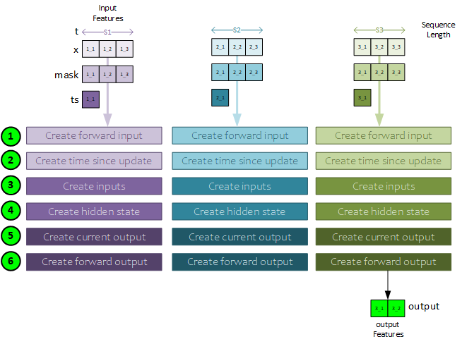
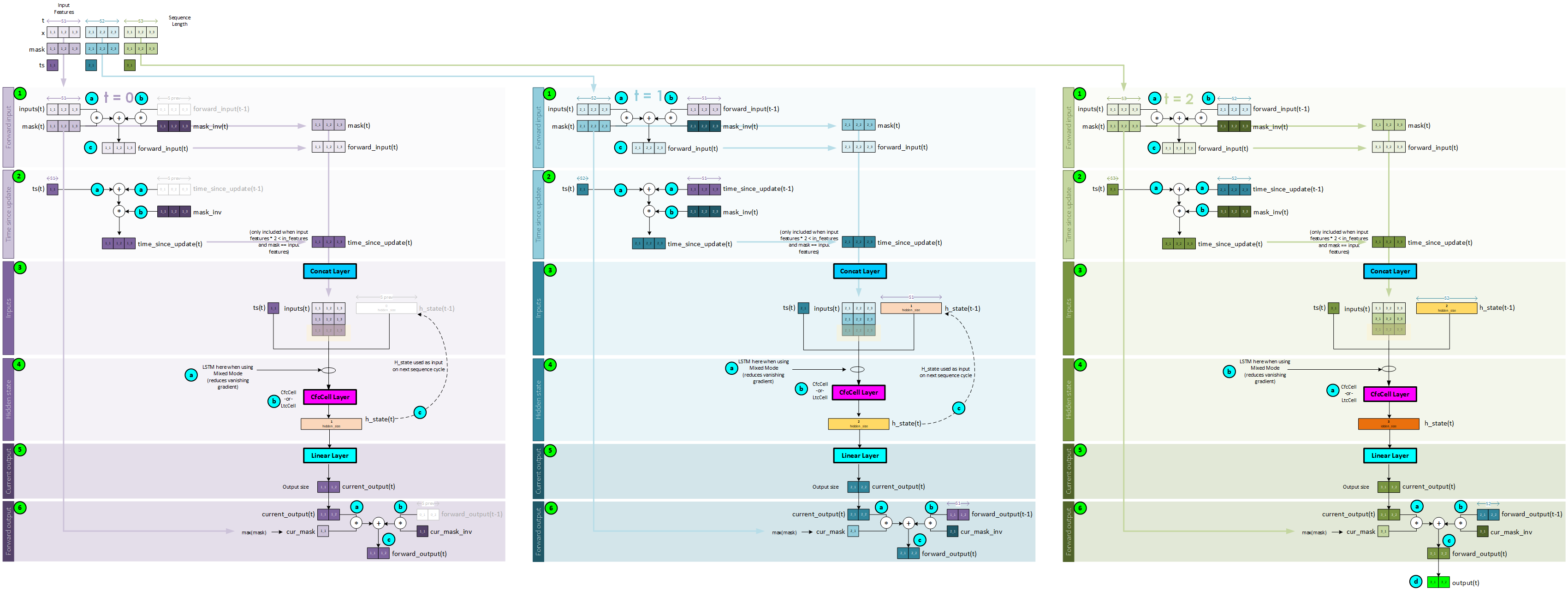
During each step in the sequence, the same processing steps occur where the processing moves from left to right through the input data. The following general steps occur during the forward pass of the CfC.

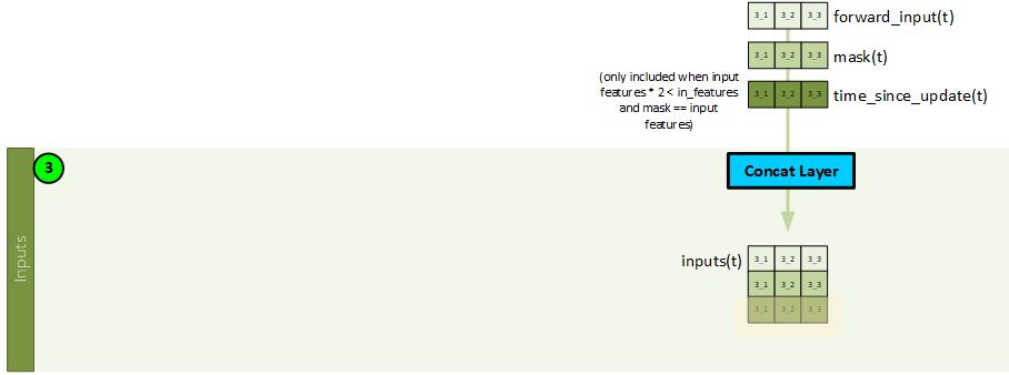
First the input for the first sequence item (t=0) is extracted from the input data and used to create the forward input, and
… the time since update. The time-since-update is used when processing 3x input features.
Next, the inputs are created by concatenating the forwarded input with the mask (and the time-since-update when processing 3x input features) – all from the current sequence item t.
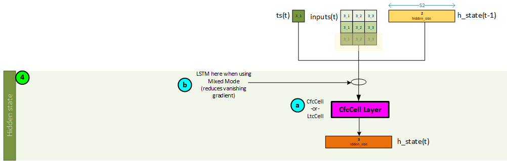
The hidden state for the current sequence item t is created by running the inputs, previous state, and time sequence through the CfCCell (or LTSCell). Note, just before running through the CfCCell the data may alternatively run through an LSTM layer first to help reduce vanishing gradients. When using an LSTM layer, the previous h state is sent to the LSTM layer and its output h state is then sent to the CfCCell.
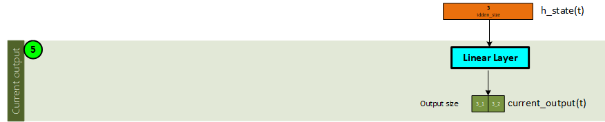
Next, the current output for the sequence item t is created by running the h state through a Linear layer.
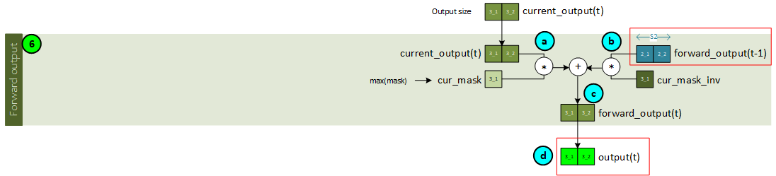
A mask is applied to the forward output and added to the mask inverse applied to the previous forward output to produce the new forward output. Upon completing the final sequence item t, the last forward output becomes the output of the CfC model containing the predictions.

The following sections show how each of these step’s work in detail.

CfC Model Processing

To better understand the processing that takes place within the CfC model, let’s step through each time sequence t in our 3 step sequence example.

First Sequence T = 0

Each of the sequences described use similar steps with several small, yet important differences.

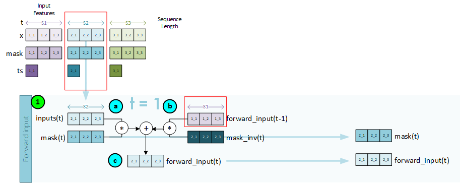
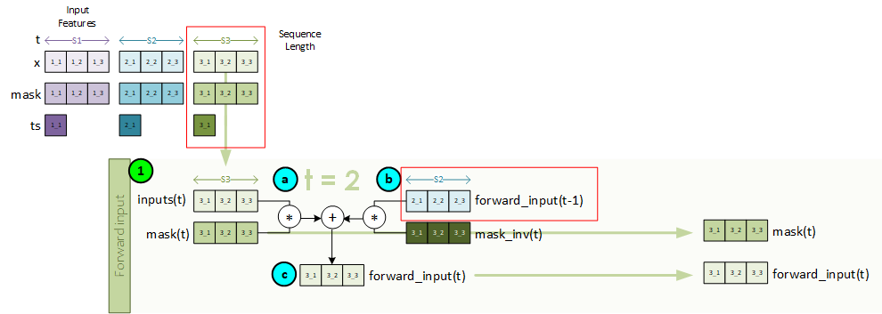
Sequence 1, Step 1 – Create the Forward Input

The forward input is created for the current step using the x and mask data associated with the first sequence item at t=0.

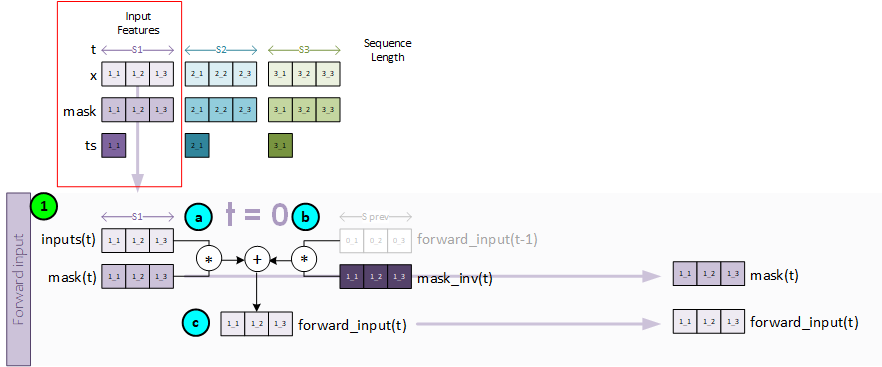
Sequence 1, Step 1 – Creating the Forward Input

To create the forward input, the following steps take place.

a. First the inputs and mask for the sequence item t are multiplied together so that we only consider the masked data.
b. Next the mask inverse is multiplied by the previous forward input, which in this case is filled with all zeros for we are at the first sequence item.
c. The new forward input is created by adding both a and b from above together.

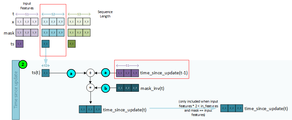
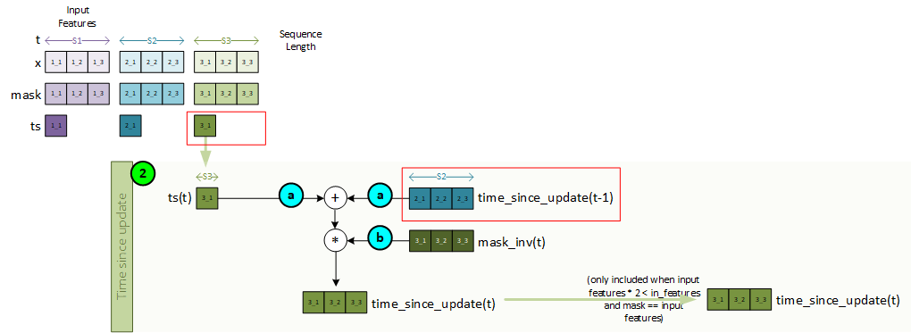
Sequence 1, Step 2 – Create the Time Since Update

The time-since-update is created for the current time step using the ts data associated with the first sequence item at t=0. Note, the time-since-update value is only used when processing 3x in-features.

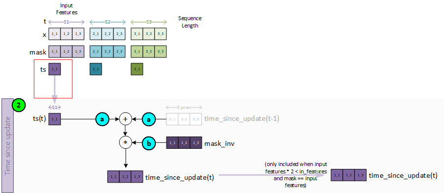
Sequence 1, Step 2 – Creating the Time Since Update

To create the time-since-update, the following steps take place.

a. The ts value for the current sequence item t is added to the previous time-since-update variable which in this case is all zeroes for we are at the first sequence item.
b. The result from a is then multiplied by the mask inverse to produce the current time-since-update value for the current sequence item t.

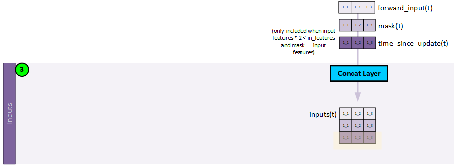
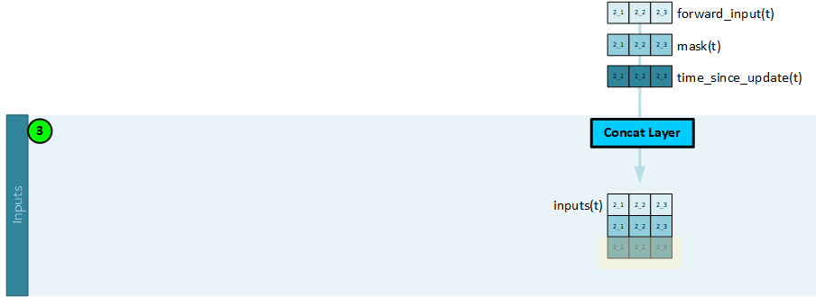
Sequence 1, Step 3 – Create the Inputs

The inputs to the cell layer (CfC or LTC) are created by concatenating the forward input and mask (and time-since-update when using 3x input features) using a Concat layer to produce the inputs for the current sequence item t.

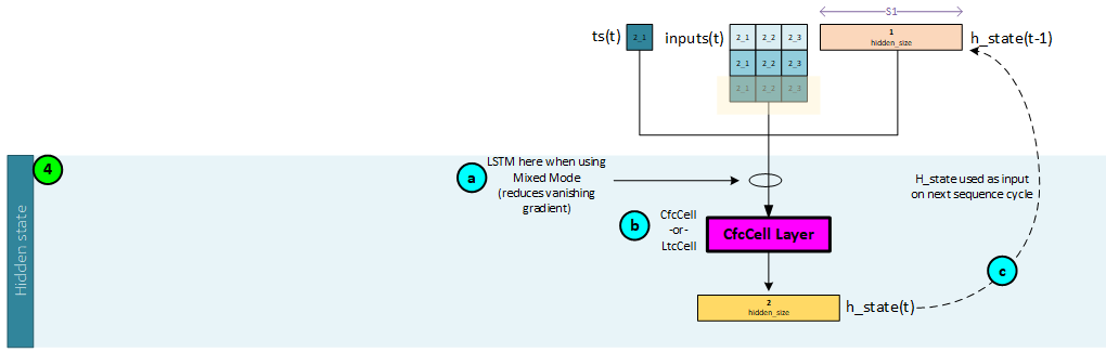
Sequence 1, Step 4 – Calculate the Hidden State

The CfC (or LTC) cell is used to create the hidden state values.

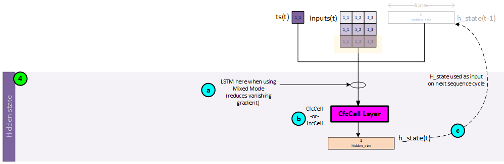
Sequence 1, Step 4 – Create the Hidden State

The following steps occur when calculating the hidden state values.

a. Optionally, the inputs (concatenated forward input, mask, and possibly time-since-update) values, previous hidden state values (from time step t-1) and previous c_state values (from time step t-1) are sent to an LSTM layer when running in mixed mode. The LSTM layer is used to help reduce a vanishing gradient. Note since this is the first time step, the previous hidden and c state values are set to all zeroes.
b. Next, the inputs are sent along with the ts and previous hidden state values (output by the LSTM layer when running in mixed mode, or from the previous time step t-1, when not) are sent to the CfCCell which produces the hidden state values for the current time step t. Note, since this is the first time step, the previous hidden state values are set to all zeroes.
c. The hidden state values output by the CfCCell become the previous hidden state values used in the next sequence processed.

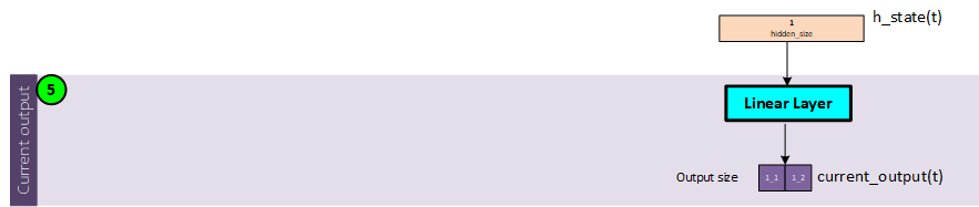
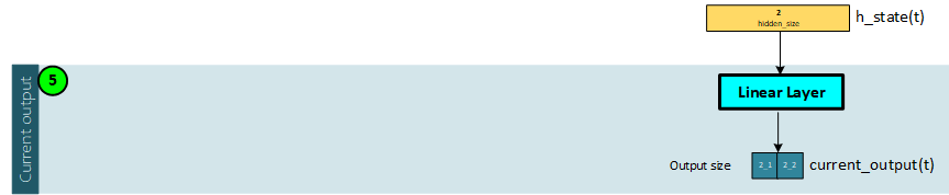
Sequence 1, Step 5 – Calculate the Current Output

A Linear layer is used to create the current output values which contain the output size of features.

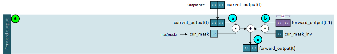
Sequence 1, Step 5 – Create the Current Output

Sequence 1, Step 6 – Create the Forward Output

The forward output is created by combining the current output with the previous forward output via masking.

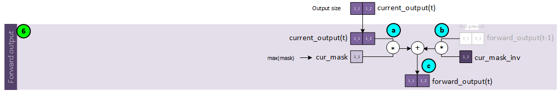
The following steps occur when calculating the forward output.

a. The current mask is calculated as the maximum of the mask for the current time step t. This current mask is then multiplied by the current output for the time step t.
b. Next, the previous forward output is multiplied by the inverse of the current mask, and …
c. … added to the result from ‘a’ above to produce the forward output for the current time step t.

Note, in the first time step, the previous forward output is set to all zeros.

At the conclusion of step 6, all processing is complete for the first time step in the sequence at t = 0. Processing now progresses to the next time step t=1 and steps 1-6 are repeated.

Second Sequence T = 1

Each sequence item t is processed using a similar number of steps as in the initial sequence t=0.

Sequence 2, Step 1 – Create the Forward Input

The forward input is created for the current step using the x and mask data associated with the first sequence item at t=0.

To create the forward input, the following steps take place.

a. First the inputs and mask for the sequence item t are multiplied together so that we only consider the masked data.
b. Next the mask inverse is multiplied by the previous forward input from time step t = 0.
c. The new forward input is created by adding both a and b from above together.

Sequence 2, Step 2 – Create the Time Since Update

To create the time-since-update, the following steps take place.

a. The ts value for the current sequence item t is added to the previous time-since-update variable from time step t=0.
b. The result from a is then multiplied by the mask inverse to produce the current time-since-update value for the current sequence item t.

Sequence 2, Step 3 – Create the Inputs

The inputs to the cell layer (CfC or LTC) are created by concatenating the forward input and mask (and time-since-update when using 3x input features) to produce the inputs for the current sequence item t.

Sequence 2, Step 4 – Calculate the Hidden State

The CfC (or LTC) cell is used to create the hidden state values.

The following steps occur when calculating the hidden state values.

a. Optionally, the inputs (concatenated forward input, mask, and possibly time-since-update) values, previous hidden state values (from time step t-1) and previous c_state values (from time step t-1) are sent to an LSTM layer when running in mixed mode. The LSTM layer is used to help reduce a vanishing gradient. Note the previous hidden and c state values are from time step t=0.
b. Next, the inputs are sent along with the ts and previous hidden state values (output by the LSTM layer when running in mixed mode, or from the previous time step t-1, when not) are sent to the CfCCell which produces the hidden state values for the current time step t. Note, the h_state values are from the previous time step t=0.
c. The hidden state values output by the CfCCell become the previous hidden state values used in the next sequence processed.

Sequence 2, Step 5 – Calculate the Current Output

A Linear layer is used to create the current output values which contain the output size of features.

Sequence 2, Step 6 – Create the Forward Output

The forward output is created by combining the current output with the previous forward output via masking.

The following steps occur when calculating the forward output.

a. The current mask is calculated as the maximum of the mask for the current time step t. This current mask is then multiplied by the current output for the time step t.
b. Next, the previous forward output is multiplied by the inverse of the current mask, and …
c. … added to the result from ‘a’ above to produce the forward output for the current time step t.

Note, the previous forward output is the forward output form time step t=0.

At the conclusion of step 6, all processing is complete for time step t=1. Processing now progresses to the final time step t=2 in our 3-time step example and steps 1-6 are repeated.

Third Sequence T=2 (Final Time Step)

Each sequence item t is processed using a similar number of steps as in the previous sequence t=1.

Sequence 3, Step 1 – Create the Forward Input

The forward input is created for the current step using the x and mask data associated with the last sequence item at t=1.

To create the forward input, the following steps take place.

a. First the inputs and mask for the sequence item t are multiplied together so that we only consider the masked data.
b. Next the mask inverse is multiplied by the previous forward input from time step t = 1.
c. The new forward input is created by adding both a and b from above together.

Sequence 3, Step 2 – Create the Time Since Update

The time-since-update is created for the current time step using the ts data associated with the last sequence item at t=1. Note, the time-since-update value is only used when processing 3x in-features.

To create the time-since-update, the following steps take place.

a. The ts value for the current sequence item t is added to the previous time-since-update variable from time step t=1.
b. The result from a is then multiplied by the mask inverse to produce the current time-since-update value for the current sequence item t.

Sequence 3, Step 3 – Create the Inputs

Sequence 3, Step 4 – Calculate the Hidden State

The CfC (or LTC) cell is used to create the hidden state values.

The following steps occur when calculating the hidden state values.

a. Optionally, the inputs (concatenated forward input, mask, and possibly time-since-update) values, previous hidden state values (time step t-1) and previous c_state values (time step t-1) are sent to an LSTM layer when running in mixed mode. The LSTM layer is used to help reduce a vanishing gradient.
b. Next, the inputs are sent along with the ts and previous hidden state values (output by the LSTM layer when running in mixed mode, or from the previous time step t-1, when not) are sent to the CfCCell which produces the hidden state values for the current time step t. Note, the h_state values are from the previous time step t=1.
c. The hidden state values output by the CfCCell become the previous hidden state values used in the next sequence processed.

Sequence 3, Step 5 – Calculate the Current Output

A Linear layer is used to create the current output values which contain the output size of features.

Sequence 3, Step 5 – Create the Current Output

Sequence 3, Step 6 – Create the Forward Output

The forward output is created by combining the current output with the previous forward output via masking. Note, in this final sequence, the forward output is also the model output containing the predicted values.

The following steps occur when calculating the forward output.

a. The current mask is calculated as the maximum of the mask for the current time step t. This current mask is then multiplied by the current output for the time step t.
b. Next, the previous forward output is multiplied by the inverse of the current mask, and …
c. … added to the result from ‘a’ above to produce the forward output for the current time step t.
d. Since we are in the final sequence step, the forward output is also the model output containing the predicted values for each of the output features.

Note, the previous forward output is the forward output form time step t=1.

Keep in mind that when processing each of the three sequences, the same CfcCell layer is used in each of the three sequence step 4’s and the same Linear layer is used in each of the three sequences step 5’s.

The full sequence processing looks as follows (click to enlarge)

CfcCell Processing

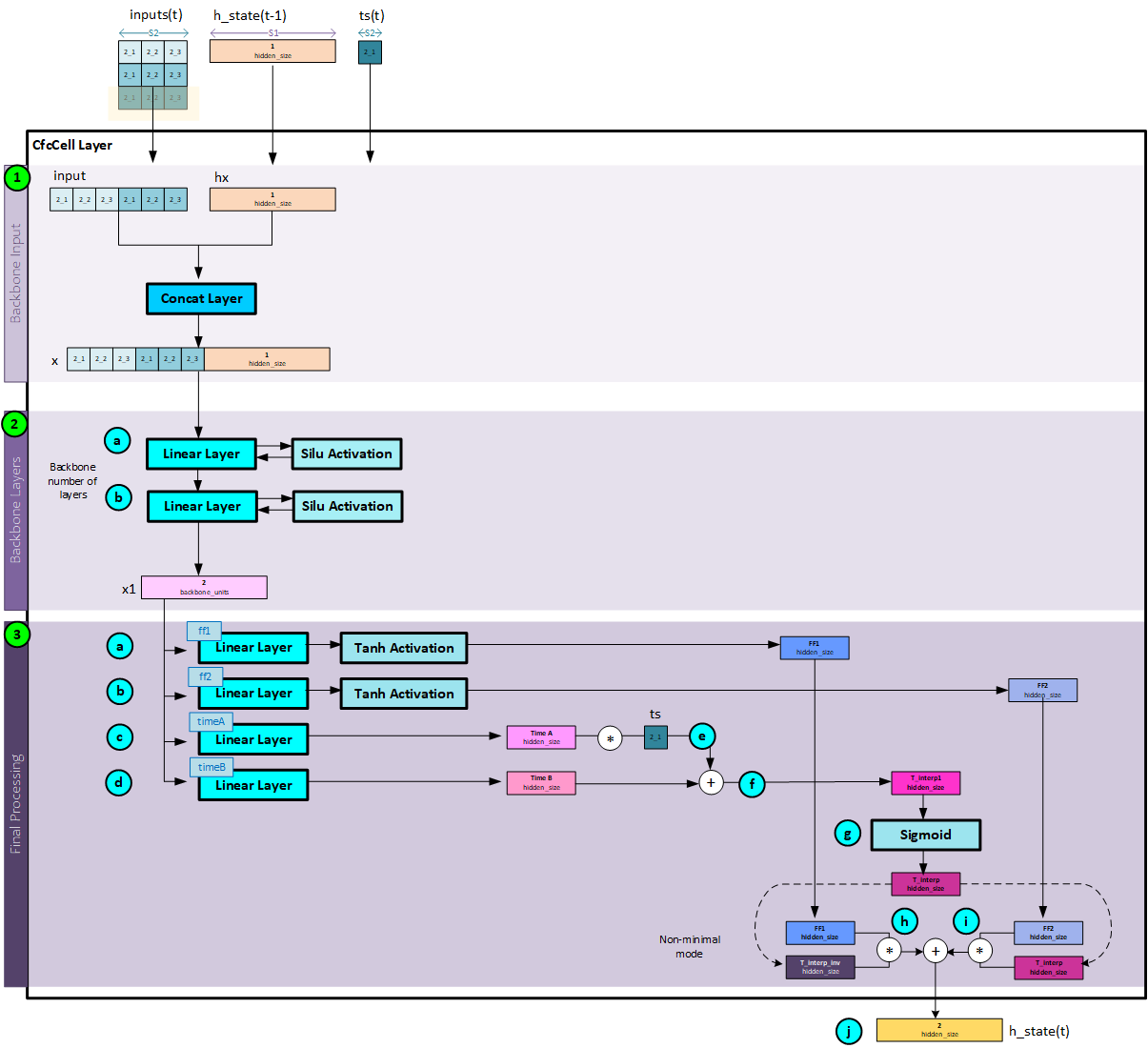
The key to the CfC model resides within the CfcCell layer. At each step with the sequence processing the CfcCell layer (or LTCCell layer) is used to calculate the hidden state that propagates forward as each sequence item is processed in time.

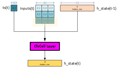
The CfcCell layer above shows an overview of the inputs and outputs produced during sequence 2 of the model. The ts, inputs and previous hidden state are fed into the CfcCell layer which then produces the current hidden state.

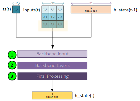
When processing the CfCCell layer, there are three main tasks that take place.

The backbone input is created by concatenating the inputs with the hidden state
The backbone input is sent through the backbone layers consisting of a set of Linear layers each followed by an activation layer such as the SiLu or ReLU
Final processing is used to combine the ff1, ff2, time A and time B outputs to produce the output hidden state.

The following sections, take a more detailed look at this process.

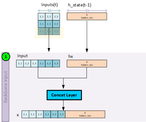
Step 1 – Create the Backbone Inputs

The backbone inputs are created by concatenating the inputs for the sequence at time step t with the hidden state from the previous time step t-1.

Step 2 – Backbone Processing

During backbone processing, the backbone inputs are run through a set of linear layers (backbone layer count), each followed by an activation unit such as the Silu or ReLU layer to produce the final backbone outputs.

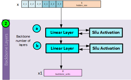
When processing the backbone units, the following steps occur.

a. The input data is passed to the first Linear layer then through an activation unit such as a SiLu or ReLU activation.
b. The output data is passed to the next Linear layer and activation unit in the backbone layers. This is repeated until all backbone layers have processed the data where the final layer outputs the x1 backbone output.

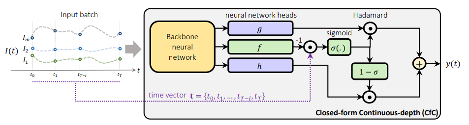
Step 3 – Final Processing

The output of the backbone neural network feeds into three head networks g, f, and h (where f utilizes two Linear layers). “f acts as a liquid time-constant for the sigmoidal time-gates of the network. g and h construct the nonlinearities of the overall CfC network.” [3]

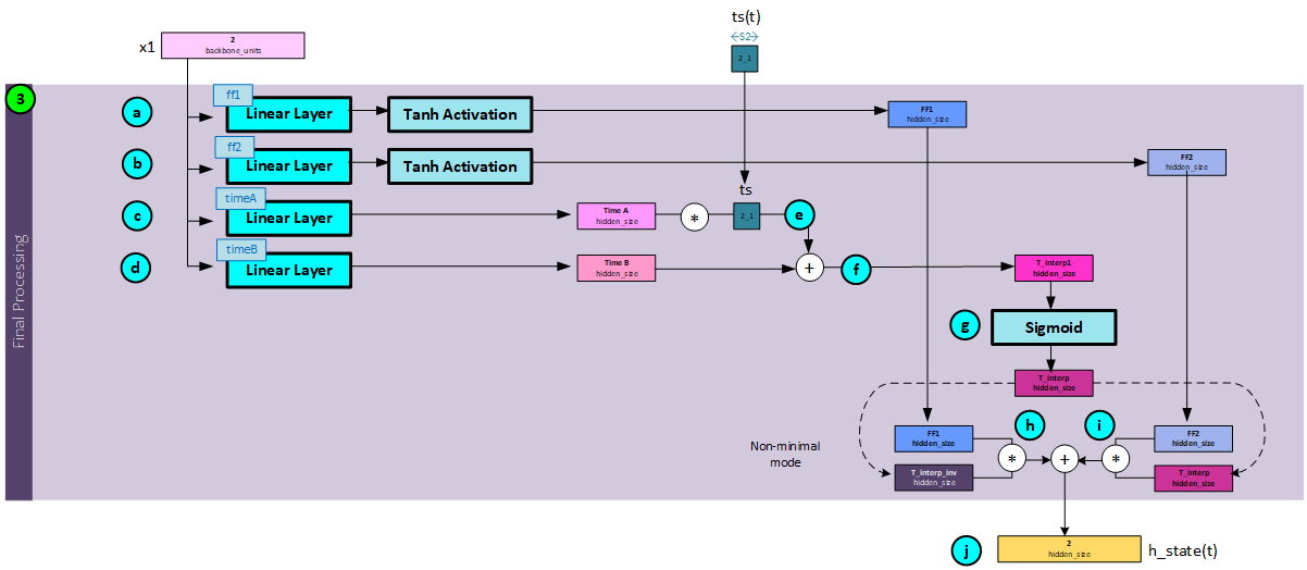
The final processing uses a set of four Linear layers used to calculate the final output hidden state for the current time step t within the sequence.

The following steps occur during the final process.

a. The backbone outputs x1 are run through the ff1 Linear layer followed by a Tanh activation to produce the ff1 Note, ff1 forms the h head gate network noted above.
b. The backbone outputs x1 are run through the ff2 Linear layer followed by a Tanh activation to produce the ff2 Note, ff2 Linear layer forms the g head gate network noted above.
c. The backbone outputs x1 are run through the timeA Linear layer to produce the timeA
d. The backbone outputs x1 are run through the timeB Linear layer to produce the timeB Note: both timeA and timeB values form the liquid time-constant for the sigmoid time gates discussed above.
e. Next, the timeA is multiplied by the current ts value for the current time step t in the sequence.
f. The timeB value is then added to the result of step ‘e’ above to produce the t_interp1 value, …
g. …, which is run through a Sigmoid layer to produce the t_interp value (σ).
h. The inverse of the t_interp value (1- σ) is multiplied by the ff1.
i. And the ff2 values are multiplied by the t_interp (σ) value.
j. The results from step ‘h’ and ‘i’ are added together to produce the current hidden state for time step t.

The full CfcCell processing looks as follows (click to enlarge)

To see the MyCaffe AI Platform code that implements the CfC model, check out the LNN Modules on our github site.

Happy Deep Learning with Liquid Neural Networks!

[1] Liquid Time-constant Networks, by Ramin Hasani, Mathias Lechner, Alexander Amini, Daniela Rus, Radu Grosu, 2020, arXiv:2006.04439

[2] GitHub: Closed-form Continuous-time Models, by Ramin Hasani, 2021, GitHub

[3] Closed-form Continuous-time Neural Models, by Ramin Hasani, Mathias Lechner, Alexander Amini, Lucas Liebenwein, Aaron Ray, Max Tschaikowski, Gerald Teschl, Daniela Rus, 2021, arXiv:2106.13898

[4] Closed-form continuous-time neural networks, by Ramin Hasani, Mathias Lechner, Alexander Amini, Lucas Liebenwein, Aaron Ray, Max Tschaikowski, Gerald Teschl, Daniela Rus, 2022, nature machine intelligence