

This post uses public documents and public data only: a mid-Columbia public utility district’s board packets, Bonneville Power Administration rate-case studies, Northwest Power and Conservation Council planning documents, USGS river gauges and EIA price history. The utility is referred to as “the PUD”; it has not reviewed this post. Every chart below carries a tag — PUBLISHED, PUBLIC FEED, MIXED or SIMULATED — and every assumption is listed in the register near the end. What is said here about how the forecast and the forward book are built today is SignalPop’s best understanding, discerned from public documents through a quantitative and probabilistic modelling lens; where a rule is inferred rather than stated, the post says so. The interactive version of every chart can be found at One Dot or the Whole Cloud Demo.
A Monte Carlo simulation [1] is the practice of answering a question about an uncertain system by drawing many plausible versions of its inputs, running the same calculation on each, and reading the answer off the distribution of results. In finance it is the standard way to value anything whose payoff depends on a path — swing options, storage, an American put [2]. In the hydro business it is also, quietly, how the region’s largest power marketer prices its rates: Bonneville runs every historical water year through its hydro simulator as equally likely — a distribution upstream — and then passes only the mean of the resulting secondary sales into the rate model [3] [4]. What the region’s public utilities do with that idea in their own budgets is simpler, and it is the subject of this post: they take the average water year, multiply by the current forward price curve, and write down one number.
This post does three things with that number. It keeps it exactly where it is. It draws the ten thousand plausible years around it. And it shows what a utility can decide once it can see them — how much energy to lock into multi-year contracts, how much of this year’s runoff to sell forward month by month, and how much to hold back — using two tools that add to the baseline rather than replace it: a correlated simulation, and a Temporal Fusion Transformer [5] that narrows the band as the year unfolds.
How a Hydro Utility Forecasts Wholesale Revenue Today
Public power utilities that own hydro typically produce a multi-year financial forecast, and the one used here is unusually well presented. Its quarterly financial review lists the wholesale revenue lines to the decimal, and its budget kickoff presentations state the method in one line, two years running: “Average water, current forward energy and carbon price curves” [6] [7]. This is not a local habit. Tacoma Power’s long-range financial plan defines its “average” case as “inflows similar to the average of all previously recorded historical water flow years” [8]. Seattle City Light’s financial forecasts “are based on average water years in the future” [9]; Idaho Power states its annual generation “under median water conditions” [10]; and a rating agency’s 2013 base case for the PUD was built “assuming average water flows”, noting in the same paragraph that regional hydrology had ranged from about 60% to 130% of average since 2000 [11].
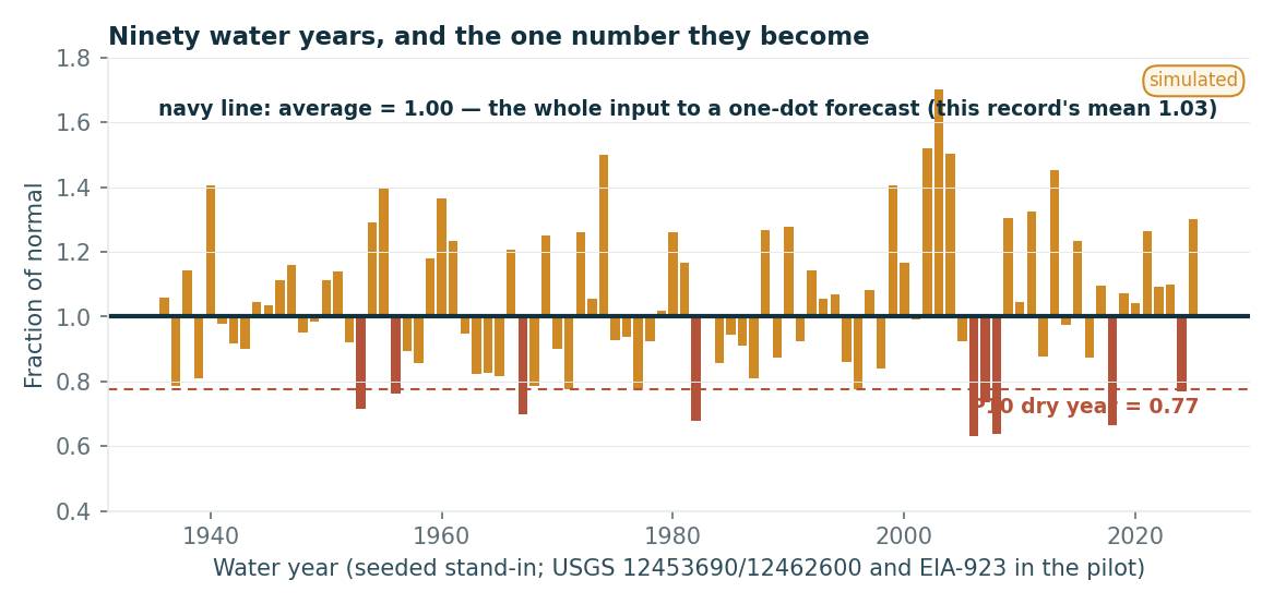
The method has a pedigree. The 90-year regional streamflow record — water years 1929 to 2018, adjusted to today’s irrigation depletions — is maintained jointly by BPA, the Corps and Reclamation [12], the Council’s GENESYS model samples the same kind of record (its 2016 documentation draws on the 80 years from 1929 to 2008) [13], and “average energy” is defined by the Council as “the amount of energy that can be expected from the hydropower system in a typical year” [14]. What follows is not a claim that any of this is wrong. It is a claim that it produces one number, and that the number is the median our model has to reproduce before it is allowed to say anything else. The current forecast method is the control.
Here is what it produces for the PUD, in millions of dollars, copied from the five-year outlook in the Q2 2026 quarterly financial review [15]:
| $M | 2026 | 2027 | 2028 | 2029 | 2030 |
|---|---|---|---|---|---|
| Service (retail) | 95.8 | 101.3 | 102.4 | 98.0 | 94.9 |
| Long-term hydro contracts | 218.4 | 213.4 | 202.8 | 194.4 | 189.4 |
| Net market-based | 109.9 | 137.8 | 177.5 | 174.9 | 185.0 |
| Other | 41.5 | 28.9 | 26.3 | 28.0 | 30.9 |
| Total | 465.6 | 481.4 | 509.0 | 495.3 | 500.2 |
| Market share of wholesale | 33% | 39% | 47% | 47% | 49% |
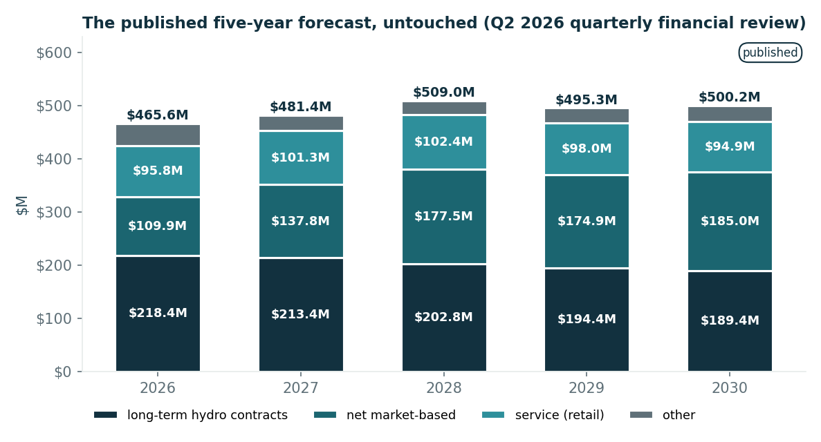
The published five-year forecast, untouched (PUBLISHED). The market-based line grows by two-thirds in four years while the contract line shrinks; by 2030 nearly half of wholesale revenue rides on the market. Two things stand out. The exposure to the market is growing, and the same review attributes the 2026 shortfall against budget to the forward price curve coming in lower than forecast. So the exposure is growing, and the method that measures it produces one number per year.
Building the Cloud
Everything that follows comes from five numbers. From the water record we measure an average (call it 1.00, a normal year) and a spread — how far a typical year lands from it. From the price record we measure the same two. The fifth number is how water and price move together across the same years: the correlation. In the Northwest it is negative — low water means the whole region is short and prices run high; high water means everyone is spilling and prices collapse. BPA’s own price study calls Northwest hydro generation “a primary driver of Mid-C electricity prices” [16], and the Council’s price forecast names hydro runoff as “a major component of price variability in the Pacific Northwest” [17]. Once the five numbers are fitted, the historical years are set aside and never drawn from again. Everything comes from the five numbers, which is worth knowing: it says exactly how much of the output is assumption.
How one dot is drawn
You do not pick a point inside an ellipse; the ellipse is what emerges after ten thousand draws. Each dot is built like this. Draw two independent standard-normal numbers, A and B. Water uses A directly. Price uses a mix: −0.45·A + 0.89·B, where −0.45 is the correlation and 0.89 is the square root of (1 − 0.45²), the leftover that keeps price’s total spread honest [18]. Then scale by each spread and exponentiate, so that water is 1.00 × exp(0.22·A) and price is $39 × exp(0.35·mixed).
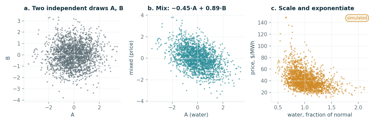
The exponentiation matters. A bell curve is symmetric and goes negative; water cannot. Working in logs makes the distribution squashed at the low end and stretched at the high end in real space, which is physically right: a drought is severe but bounded, a flood year has no natural ceiling.
Two limits of the recipe are worth stating before the code. A lognormal is strictly positive. That is right for an annual average, which has never been negative at Mid-C, but hourly and daily prices do go negative in spring runoff, so the forward-book and day-ahead valuation in the pilot uses a price process that allows negative prices and spikes. And the published dot is placed at the median of each draw. A log normal’s arithmetic mean sits σ²/2 above its median — about 2.4% for water at σ = 0.22 and 6.3% for price at σ = 0.35 — so if the utility’s published figures are means rather than medians, the whole cloud shifts down by that much. The pilot fits the shape from the record and settles which it is; the acceptance test is the same either way.
In code, the whole draw is short:
import numpy as np

n, sig_w, sig_p, rho = 10_000, 0.22, 0.35, -0.45
P0 = 109.9 / 2.8                     # $/MWh implied by the published 2026 market line
A, B = np.random.standard_normal((2, n))
water = np.exp(sig_w * A)                                # fraction of normal, median 1.00
price = P0 * np.exp(sig_p * (rho * A + np.sqrt(1 - rho**2) * B))
The price center, $39.25/MWh, is not an opinion. It is the price the published 2026 market line implies once the volume is reconstructed: $109.9M divided by 2.8 million MWh. EIA’s Mid-Columbia history averages closer to $43 over 2010–2025 [19]; the forward curve the PUD used is lower, and we take the PUD’s number, because the current forecast method is the control.
The cloud
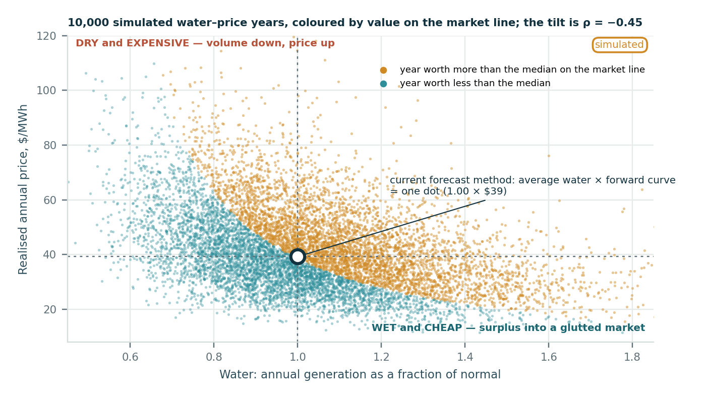
Read the tilt as physics rather than statistics. Low water means less hydro on the regional market, supply is short, price runs high. High water means everyone is spilling, the region is swimming in cheap power. A flat cloud would claim that water tells you nothing about price — a strange claim for a river that is a large share of regional supply. The consequence for the utility is that keeping energy uncommitted is a hedge, not a gamble: in the years when there is less to sell, each unit sells for more. A fixed-price contract signed at the forward curve gives that hedge away, and a single forward curve cannot represent it, because a single curve has one price regardless of what the water did.
One dot becomes one revenue number
Each dot is turned into a revenue number with the utility’s own spreadsheet arithmetic, unchanged. The dot’s water value is a bare ratio, say 0.91. Multiply by average annual generation — 9.0 million MWh, the PUD’s own published figure — and this simulated year produced 8.19 million MWh. Retail load (about 2.6 million MWh) is served first at fixed rates; it is demand, not a destination for surplus. The cost-based contracts are served next, and they are slices: the buyer takes a percentage of actual output, so contract volume scales with the river (3.6 million MWh in a normal year). Whatever is left — roughly 2.3 million MWh in this dot — is the merchant slice, the only part valued at the dot’s price. Add back the revenue that is the same in every dot — retail rates, the contract price of $60.7/MWh implied by $218.4M over 3.6 million MWh, and “other” — and that is one revenue outcome.
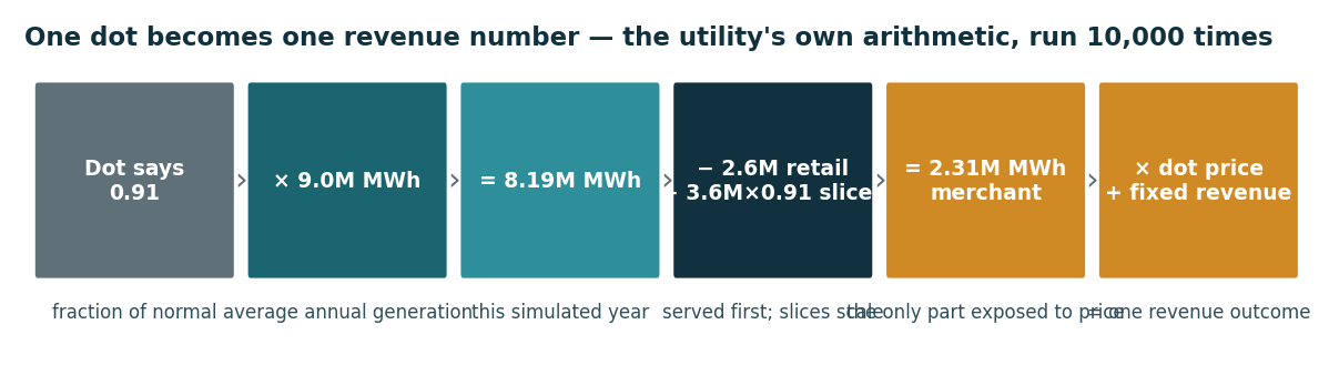
GEN, RETAIL, LT = 9.0, 2.6, 3.6           # million MWh; 3.6 and 2.8 are reconstructed volumes
merchant = np.maximum(GEN * water - RETAIL - LT * water, 0)
market_rev = merchant * price               # $M, the only line exposed to price
total_rev = 95.8 + 41.5 + 218.4 * water + market_rev
Two honesties are owed here. The two volumes (3.6 and 2.8 million MWh) are reconstructed so that the arithmetic reproduces the published $218.4M and $109.9M lines; they are the first thing to ask staff for. And the merchant slice is leveraged: retail does not shrink in a dry year, so a 10% water miss lands almost entirely on the uncommitted energy, which is why the size of the committed book is itself the decision worth the most money.
Sort the list. The sorted list is the product.
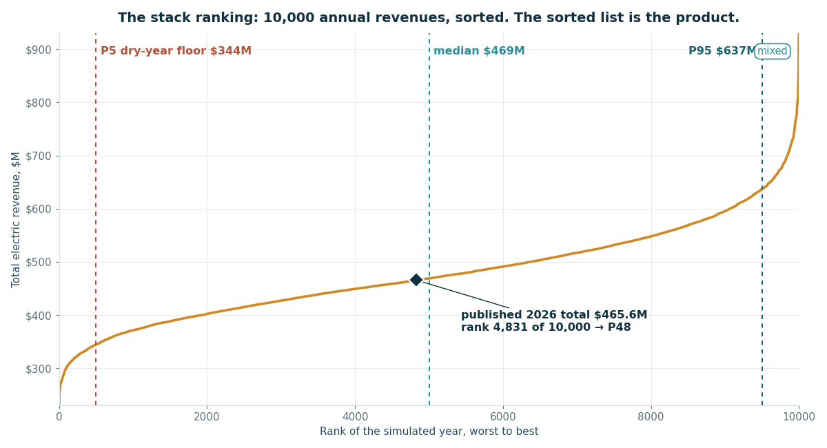
Ten thousand revenues, sorted. Count five hundred in from the bottom and that is the P5 dry-year floor, $344M. The middle is the median year, $469M — half the years are better, half worse. Five hundred from the top is the good case, $637M. And the published 2026 total of $465.6M lands at rank 4,831 — the 48th percentile. That is the single best first slide in any conversation about this method, because it says two things at once: the model reproduces the current forecast method almost exactly, and there is a range $293M wide around it that nobody has been able to see. If the published number had landed at the 60th percentile it would mean the planning number is mildly optimistic, beaten in four years out of ten. Either result is useful, and neither is “your number is wrong.”
How today’s haircut splits the same years
The sorted list also shows something the forward book does every month without drawing it. The desk does not sell the whole expected surplus forward; it applies a haircut, committing only the volume that would exist under a conservative water case, and lets the rest ride to the day-ahead and real-time market. The convention is documented across the region. Bonneville commits only “firm” generation, defined as the monthly tenth percentile of the record, and treats “generation from water in excess of critical water conditions” as secondary energy “valued at expected wholesale market prices … at the Mid-Columbia (Mid-C) trading hub” [27] [28]. Tacoma Power’s rate policy plans surplus sales on water “exceeded 75 percent of the time” [29]. Seattle City Light “maintains strict limits on the portion of its surplus position made available for forward sales to avoid potentially high replacement power costs in low-water years” [30]. And the PUD’s own 2011 resolution caps net forward sales within the year at “the annual surplus energy at the 50th percentile level as determined from the District’s probabilistic simulation model” [31] — which is worth pausing on: the desk already has a water distribution. What that cap does not carry is price drawn jointly with water, or a stated tolerance for being short. (Its medium-term hedges are also slices, which pass volume risk to the buyer [32]; the fixed block below is the forward-book analogue, not the slice book.)
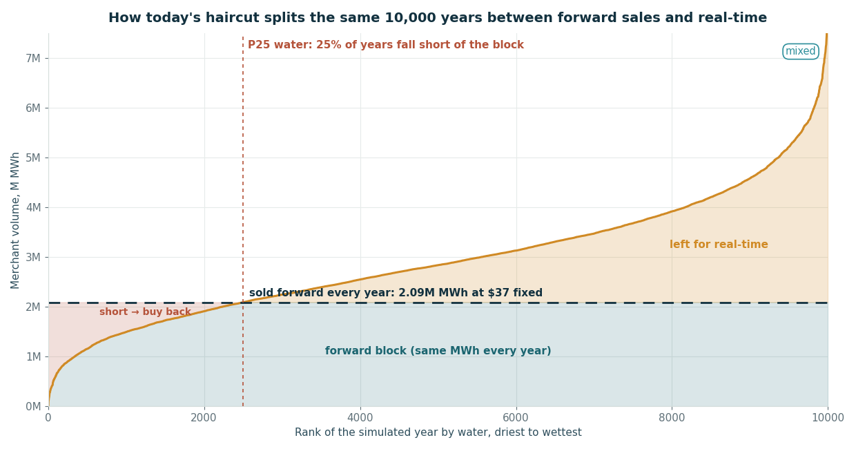
At a P25 haircut the block is about 2.1 million MWh, worth about $78M a year at the forward price; the remainder averages $36M of real-time sales, a third of merchant revenue, most of it earned in wet years when prices are low; and in the driest quarter of years the shortfall is bought back at an average cost of $7.7M a year. The haircut is a fixed percentile. It does not move with what is known about the year, and it is not tied to any stated tolerance for being short. Both of those are things a distribution can fix, and the second of them is where the forecasting model earns its place.
What a better-conditioned dot is worth
Suppose that at the time of commitment a forecaster had already resolved part of this year’s water uncertainty — from snowpack, soil moisture, the river forecast center’s outlook — and the block were sized from that distribution instead of the climatological one. To isolate what the forecaster adds, hold the shortfall frequency fixed: the forecaster sizes its block at the conditioned P25, so both rules are short in about one year in four and every dollar of difference is the forecaster’s. At zero skill the two rules are, by construction, the same rule.
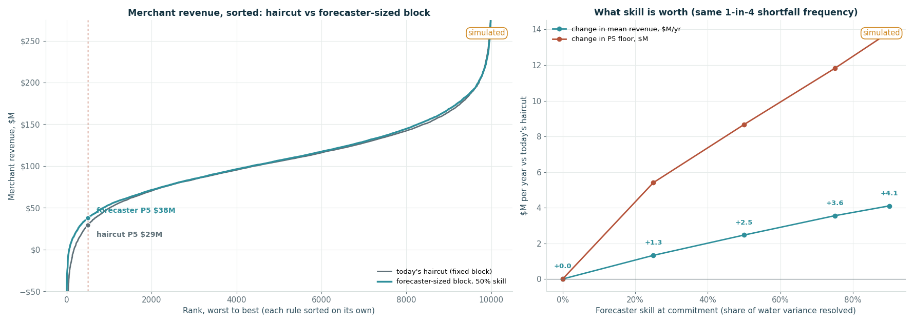
With half of the year’s water uncertainty resolved at commitment, average merchant revenue rises by about $2.5M a year and the dry-year floor by about $8.7M, from $29M to $38M; at 90% skill the figures are $4.1M and $14M. The gain is not from being right about the year. It comes from committing more in the years the forecaster can already see are wet, where the alternative was dumping energy into a cheap spot market, and less in the years it can see are dry, where the alternative was buying it back in a dear one. Choosing the tolerance itself — one short year in twenty rather than one in four — is a second and separate gain, sized later in this post. Skill is the placeholder in this chart, and it is the one thing a simulation cannot supply: it comes from a model built on the real drivers and proven in a walk-forward backtest.
Reading the Sorted List
Every question after this is answered by changing something, re-running, and watching the two numbers that matter — the floor and the median — move. Because the whole model rests on five numbers, the most important thing to do with it is stress the fifth one. Here is the same sorted list under four correlations, everything else unchanged:
| Correlation ρ | Total P5 | Total P50 | Total P95 | Market line P10–P90 |
|---|---|---|---|---|
| 0.00 (no lean) | $332M | $469M | $692M | $50M – $218M |
| −0.20 | $337M | $469M | $668M | $54M – $202M |
| −0.45 (base) | $344M | $469M | $637M | $60M – $180M |
| −0.70 | $354M | $468M | $606M | $68M – $158M |
The median does not move; the correlation is not a knob for the headline. What it does is narrow the band from both ends — the river hedges itself a little, and the stronger the lean the more it hedges. That reframes the correlation slider on the interactive page from “look what I can make the answer do” to “here is how much the answer depends on the thing I have already stress-tested.” A trillion draws would map the ellipse beautifully but could never produce something the recipe does not contain: if the real world has fatter tails than lognormal — droughts deeper than the record, a 2021-style price spike — the model will not invent them — and the peer-reviewed literature makes the same point about the region’s own expected-value hydro planning [26]. Hence the companion exhibit nobody can argue with: replay all ninety historical years against today’s book. No simulation, no shape assumption, just what actually happened.
Where the Temporal Fusion Transformer Adds to the Baseline
Everything so far works with any reasonable distribution, and none of it uses machine learning. The cloud is drawn from ninety years of climatology, so it says the same thing every October regardless of what the mountain looks like. That is where a forecasting model earns its place, and it is worth being precise about what it adds and what it does not.
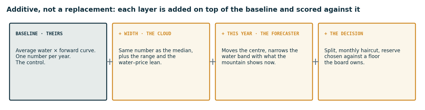
The baseline is the current forecast method, and it is the control. The cloud adds width: the same number as the median, plus the range and the water–price lean, which is what gives the board a dry-year floor to own. The forecaster adds this year: it moves the center and narrows the water band with what the mountain shows now. The decision layer adds a split, a monthly haircut and a reserve chosen against that floor. The value of the forecaster is measured the only honest way — the same forecast made from 1 January of each past year using only what was knowable then, scored against what happened, side by side with the ninety-year average as the naive baseline [20]. The gain is the difference. If the backtest shows none, the baseline stands and the cloud alone still carries the decision. Nobody is asked to concede that their point forecast is inaccurate, because that is not the claim: the claim is that it is conditioned on long-run averages, and a walk-forward test shows whether conditioning on current information helped historically.
A Temporal Fusion Transformer [5] suits this problem unusually well. It is built for multi-horizon forecasting with a mix of known-future inputs (calendar, scheduled outages, contract step-dates), observed inputs (snowpack, gas price, recent inflow) and static ones (plant, unit); it emits quantiles at every horizon rather than a point; and its variable-selection weights give an interpretable account of which inputs the forecast leaned on — an interpretability aid, not a causal explanation. It is trained on the real record only — snowpack, weather, flows, gas and power prices, and what happened next — and never on the simulated dots, which would be circular. Its output feeds into the simulation as conditioning: instead of drawing from ninety-year climatology, draw from “given what the mountain looks like today.”
It is worth being plain about why this is the part that matters, and the part that is hard. The cloud is honest, but anyone with a statistics package can draw it, and the PUD’s own resolution shows a probabilistic surplus model already exists on the desk [31]. What no one on the river has is the conditioned dot: a forecast of this year’s water and price, at every horizon from a week to eighteen months, that carries its own calibrated width and can report which inputs it leaned on. That is a different kind of object. It has to learn from many related series at once — snowpack at a dozen SNOTEL sites, soil moisture, temperature outlooks, gas, the river forecast center’s own numbers — while respecting inputs that are known in advance; it has to emit quantiles so it can be scored; it has to be tested walk-forward with no leakage from revised datasets; and it has to attribute its forecast to inputs a commissioner can repeat. The Temporal Fusion Transformer was designed for exactly that combination [5], and SignalPop implemented it natively in its own deep-learning framework, MyCaffe, in 2023 [33] and runs transformer-based probabilistic forecasters in production on live financial data, where a mis-stated width costs money the same afternoon. The skill chart above puts a dollar figure on whatever skill the backtest proves; building the thing that earns the skill is the work.
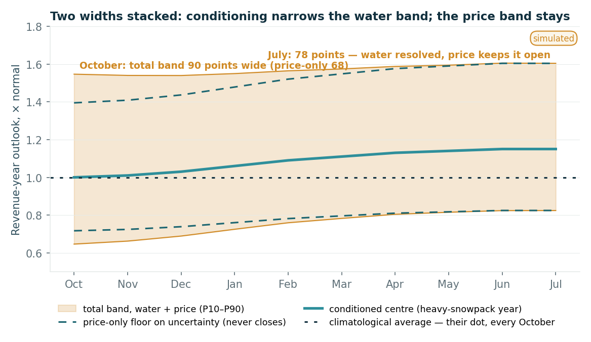
Two things to notice. The band in October is about 90 points wide (P10 to P90, as a multiple of a normal revenue year); by July it is still nearly 80, because water uncertainty is only part of it and price uncertainty is the part that stays. And the center moves: in an unusual year, by spring, the conditioned forecast and the climatological dot are materially different, and that is where the near-horizon money is. Over a twenty-year contract this year’s snowpack barely matters — the cloud sells the long-horizon decision; the forecaster sells the near-horizon one.
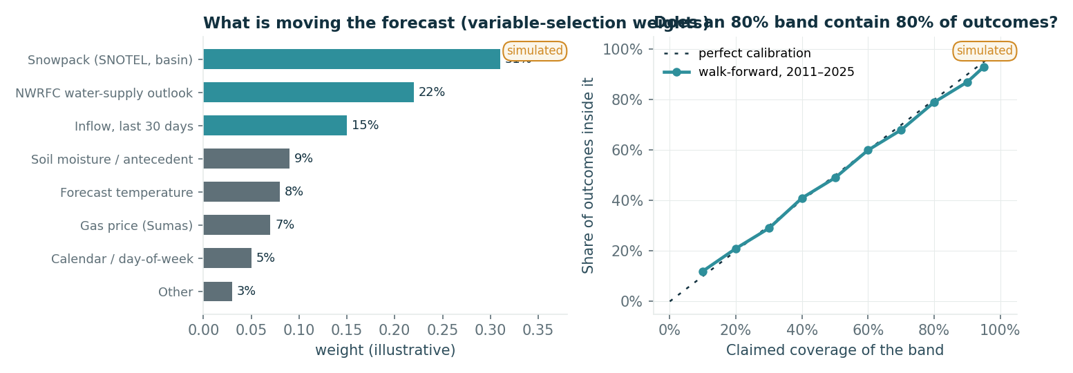
The two panels are what make a probabilistic forecast defensible in front of a board. The attribution weights say which inputs the forecast leaned on, in terms a commissioner can repeat — snowpack, the river forecast center’s outlook [21], recent inflow, gas. And the calibration curve is the test a point forecast cannot fail: if the model claims an 80% band, do 80% of outcomes land inside it, year by year, walking forward? Calibration and sharpness together are the proper score for a probabilistic forecast [20]; a forecast that is calibrated but no sharper than climatology has added nothing, and the backtest says so. The transformer is the right tool out to about eighteen months; beyond that it is extrapolating, and a calibrated stochastic process with a long hydrology bootstrap [22] takes over for contract-term horizons.
Deciding What to Sell Forward and What to Keep
Three decisions change once the forecast has width, and all three depend on the same two things: how wide the band is right now, and whether water and price still lean against each other.
Is the lean stable?
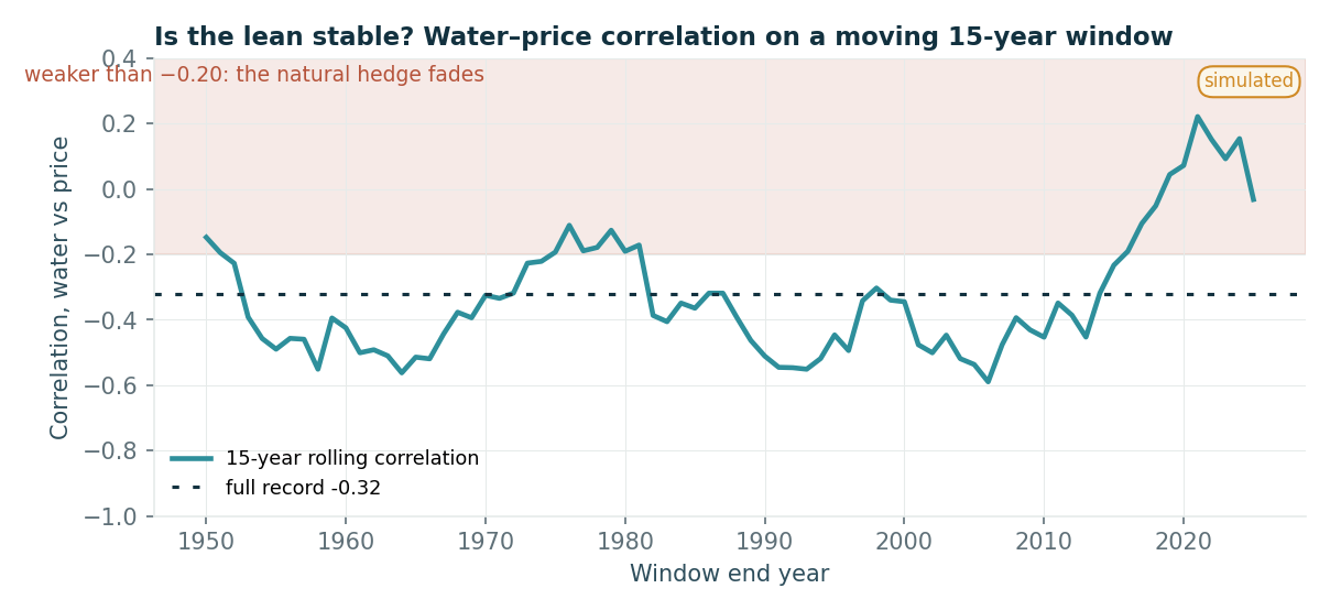
The correlation is the number the decision leans on most, so it should be fitted on rolling windows and shown drifting, not asserted. Time-varying correlation has its own estimators [23]; the moving window is the version a room can read. If the lean is stable, it is a quantified natural hedge you can put a dollar figure on. If it drifts, the split is chosen so that it survives every regime in the window — robustness rather than prediction. Either answer helps, and the stress test is the strongest room answer.
How much of this year’s runoff to sell forward
The desk logic on the forward book, as documented across the region and inferred for the PUD [27]–[31], is to start with expected volume for the month, take a haircut so you are not selling water you might not have — against a conservative water case, by convention rather than calculation — compare the forward price to budget, and sell if it looks decent. That rule has a weakness that is easy to state: it is not tied to any tolerance. Nobody has said what probability of being short is acceptable, and the same haircut is applied in October, when nothing is known about the year, and in May, when most of it is.
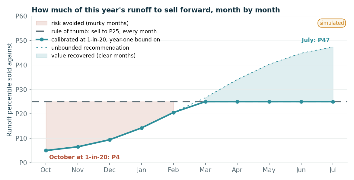
The product in one sentence: the board sets the tolerance once (“short in no more than one year in twenty”); each month the model works out what volume satisfies it given how far the forecaster has narrowed the band — less than the old haircut in a murky month, more in a clear one. The governance shape is the same as everywhere else in this post: staff own the tolerance, the model finds the number, and the rule stops being a fixed percentage inherited from whoever set it. And the year-one clause is what makes it safe to adopt: the model may recommend selling less than the current rule, never more, so the worst case is never worse than today’s practice.
How much to lock in
The PUD’s hedging policy has historically targeted a fixed share of sales under cost-based contracts. A share is a reasonable rule of thumb, and it was chosen without a curve to choose from. Take the energy that has actually come free to re-allocate — about 0.9 million MWh a year by 2029 as contracts roll off — and value every split between a multi-year fixed-price commitment and energy kept flexible for forward and day-ahead sale, on the same ten thousand years.
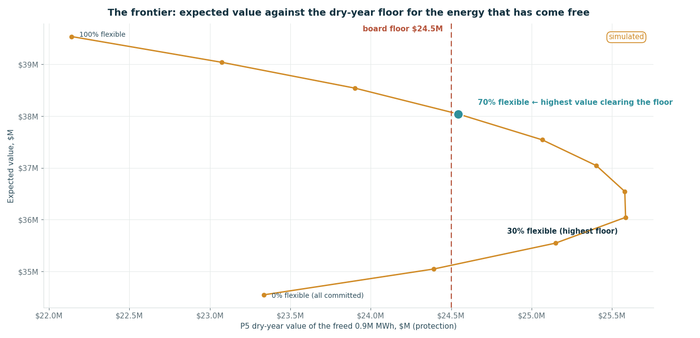
Two features of the curve are worth a commissioner’s attention. Expected value rises with flexibility, as it should — the flexible side sells at the dot’s price with a modest shaping premium, the committed side at a discount to the forward. But the dry-year floor rises too, up to about 30–40% flexible, before price risk takes over. That shape is a property of the correlation, not an opinion: keeping some energy uncommitted raises the worst-year outcome because dry years sell dear. Set the correlation to zero on the interactive page and the bulge disappears. Set the floor the board is willing to own and the split falls out; on these placeholders, at a floor of $24.5M the answer is to keep more flexible than a fixed-share rule would — and to be able to say why.
The third decision — the reserve — uses the same machine with one extra check per dot. The Western Resource Adequacy Program becomes binding for every participant from the winter 2027–28 season, which begins 1 November 2027; summer 2027 is an optional early binding season [24]. Its obligation is a forward showing of qualifying capacity, in megawatts, for the season’s critical hours — not a subtraction of annual energy — and what counts toward it depends on qualifying resources, qualifying contracts and transmission rights, so a fixed-volume forward block can constrain what the utility is able to show. “Hold enough” is a rule of thumb; “hold enough that the probability of being short in any binding hour is below the tolerance” is a number, read off the distribution, and it is usually a smaller one. That question needs the monthly and hourly version of the model — twelve means, twelve spreads and a month-to-month correlation table so that a bone-dry April is never followed by a record May — which is the natural scope of a pilot rather than a public page.
Assumptions and Data
Four kinds of number appear in this post, and it should be possible to tell which is which at a glance.
| Quantity | Value used | Kind | Source / how it is replaced |
|---|---|---|---|
| Revenue lines 2026–2030 | as tabulated | Published | PUD Q2 2026 quarterly financial review, five-year outlook [15] |
| Forecast method wording | quoted | Published | PUD 2025 and 2026 budget kickoff decks [6] [7] |
| Average annual generation | 9.0M MWh | Published | PUD fast facts; EIA-923 for the plant-level series (plant IDs 3883, 6200 and 6424)[19] |
| Retail load | 2.6M MWh, held constant | Reconstructed | Clean-energy compliance-period forecast ÷ 4; pilot models it as a third correlated variable |
| Cost-based contract volume | 3.6M MWh, scaling as a slice | Reconstructed | Chosen so $218.4M ÷ 3.6M = $60.7/MWh; first item on the data request |
| Market volume; implied price | 2.8M MWh; $39.3/MWh | Reconstructed | 9.0 − 2.6 − 3.6; $109.9M ÷ 2.8M MWh; cross-check EIA Mid-C mean ≈ $43 |
| Water spread σw | 0.22 | Placeholder | Fit on USGS 12462600 water-year discharge [25] and EIA-923 |
| Price spread σp | 0.35 | Placeholder | Fit on EIA/ICE Mid-C annual averages; flat average, no on-peak weighting (a floor) |
| Correlation ρ | −0.45 | Placeholder | Fit on the deseasonalised monthly record with a confidence interval; direction supported by [16] [17] |
| Distribution shape | lognormal, Cholesky mix; published dot at the median | Method | [18]; fat tails and negative prices not generated; mean sits σ²/2 above the median (2.4% water, 6.3% price) — the pilot fits mean-corrected or empirical marginals and a price process with negative prices; the historical replay against today’s book is the companion exhibit |
| The ninety water years | seeded synthetic | Placeholder | USGS 12462600 daily discharge (June 1961 on) aggregated to water years — 12453690 has no discharge record (stage and reservoir elevation only); the 2020 Level Modified Streamflow record [12] |
| Knowledge schedule (band narrowing Oct→Jul) | 0% → 96% resolved | Placeholder | The forecaster’s own walk-forward quantiles; SNOTEL and NWRFC inputs [21] |
| Year types, attribution weights, calibration curve | illustrative | Placeholder | Produced by the trained model and its backtest |
| Forward-book rule of thumb (haircut) | sell forward the merchant volume at P25 water | Assumption | Regional convention documented at P10 (BPA firm), P25 (Tacoma) and the PUD’s P50 cap from its own probabilistic surplus model [27]–[31]; replaced by what the desk actually uses |
| Forecaster skill at commitment | 0–90% of water variance resolved | Placeholder | Produced by the walk-forward backtest against the ninety-year average; the chart shows the value of whatever skill is proven |
| Freed energy | 0.9M MWh/yr by 2029 | Reconstructed | Roll-off of contracts expiring end-2026 and end-2028; pilot uses actual terms |
| Fixed-price discount; shaping premium | 5%; 6% | Placeholder | Measured against captured price vs flat average; applied only to flexibility actually controlled after fish, flow and coordination constraints |
| Fleet; resolution | one machine; annual | Simplification | Unit-level history and outage log; monthly correlated draw for the reserve and forward-book questions |
The rule for every number: it is either the PUD’s, public, or labelled as a placeholder that the pilot replaces. Nothing is presented as a result that has not been computed, and nothing is presented as a result at all — the distributions are placeholders and the levers are illustrative. What is real is the arithmetic, the published lines it reproduces, and the shape of the decision.
Summary
A hydro utility’s revenue forecast is built the way the whole region builds them: average water, current forward curve, one number per year, and there are good public documents saying so. Keeping that number as the median and drawing the ten thousand plausible years around it — with the water–price lean preserved, using the utility’s own arithmetic — reproduces the published forecast almost exactly and reveals a range nearly $300M wide that nobody had been able to see. Sorting the list gives the board a dry-year floor to own; stressing the correlation shows how much the floor depends on the river hedging itself. A Temporal Fusion Transformer [5] [33] adds to that baseline rather than replacing it: it moves the center and narrows the water band with this year’s conditions, emits quantiles that can be scored for calibration, and reports which inputs it leaned on through its variable-selection weights — and it earns its place only by beating the ninety-year average in a walk-forward backtest. With the width and the lean in hand, three rules of thumb become three numbers: the share to lock in, the monthly haircut on the forward book, and the reserve to hold. In every case the board keeps the tolerance, and the model finds the number.
The interactive version — the cloud, the stack ranking, the haircut split and the forecaster slider, the published forecast, the fan, the moving-window correlation and the frontier, with every slider labelled as a stress test — is at One Dot or the Whole Cloud Demo. To discuss how this could benefit your site, request a 90-minute walkthrough: Contact Us.
Happy simulating on the river!
[1] Monte Carlo Methods in Financial Engineering, by Paul Glasserman, 2003, Springer (Stochastic Modelling and Applied Probability 53)
[2] Valuing American Options by Simulation: A Simple Least-Squares Approach, by Francis A. Longstaff and Eduardo S. Schwartz, 2001, The Review of Financial Studies 14(1):113–147
[3] BP-22 Power Market Price Study and Documentation (BP-22-FS-BPA-04), by Bonneville Power Administration, July 2021 — “HYDSIM produces 80 year-long records of PNW monthly hydroelectric generation, based on actual water conditions in the region from 1929 through 2008”; each iteration samples one of the 80 water years “from a discrete uniform probability distribution.”
[4] BP-26 Power Rates Study (BP-26-FS-BPA-01), by Bonneville Power Administration, July 2025, §2.1.6.8 — “Mean prices and quantities of these secondary sales, as well as mean market prices, are passed to RAM2026 for the purposes of the secondary revenue credit.”
[5] Temporal Fusion Transformers for Interpretable Multi-horizon Time Series Forecasting, by Bryan Lim, Sercan Ö. Arık, Nicolas Loeff and Tomas Pfister, 2021, International Journal of Forecasting 37(4):1748–1764; arXiv:1912.09363
[6] 2025 Budget Kickoff, the utility’s public board packet, October 2024, “Key 2025 Budget Assumptions — Wholesale Revenue”: “Average water, current forward energy and carbon price curves; hedge program fully implemented and continuing.”
[7] 2026 Budget Kickoff — Timeline and Key Assumptions, the utility’s public board packet, October 2025, under Net Market-Based Energy Revenue: “Average water, current forward energy and carbon price curves.”
[8] Long-Range Financial Plan 2024, by Tacoma Power, pp. 23–24 — “Average: Inflows similar to the average of all previously recorded historical water flow years”; Tacoma budgets on its “Adverse” case, “inflows similar to the lowest 25% of recorded historical years.”
[9] River Conditions Improve, Lift City Light’s Financial Forecasts, by Seattle City Light (Powerlines), 21 July 2014 — “Those forecasts are based on average water years in the future.” See also Strategic Plan Financial Forecast Assumptions 2022–2026, p. 12, net wholesale revenue “based on expected prices and normal hydro conditions.”
[10] Form 10-K for the fiscal year ended December 31, 2016, by IDACORP, Inc. / Idaho Power Company, 2017, Item 1 — “annual generation of approximately 8.5 million Megawatt-hours (MWh) under median water conditions.”
[11] Rating-agency credit report on the PUD, February 2013 (public on the utility’s site) — “Assuming average water flows, the all-in weighted average production costs are expected to be around $17/MWh by 2016”; regional hydrology “reaching a low of around 60% of average and a high of around 130% of average since 2000.”
[12] 2020 Level Modified Streamflow, 1928–2018 (DOE/BP-4985), by Bonneville Power Administration with the U.S. Army Corps of Engineers and the Bureau of Reclamation, October 2020 — 90 years of flows adjusted to 2018 irrigation depletions
[13] GENESYS Technical Documentation, by Northwest Power and Conservation Council, 11 October 2016, §3.2 — “An 80-year historical record of streamflows from 1929 to 2008 is sampled.”
[14] Draft Fourth Northwest Power Plan, Appendix A, by Northwest Power and Conservation Council, p. A-3 — “average energy” is “the amount of energy that can be expected from the hydropower system in a typical year.”
[15] Quarterly Financial Review, six months ended 30 June 2026, presented to the commission 3 August 2026, five-year outlook and “key modeling assumptions” appendix (“past water history and current forward price curve”). The utility’s published quarterly financial report for the same period is public; the review slides are in the 3 August board packet.
[16] BP-26 Power Market Price Study (BP-26-FS-BPA-04), by Bonneville Power Administration, July 2025 — “PNW hydro generation is a primary driver of Mid-C electricity prices”; 2,700 iterations each sampling one of 30 water years (1989–2018) uniformly
[17] 2021 Northwest Power Plan: Wholesale Electricity Price Forecast, by Northwest Power and Conservation Council, 2022 — hydro runoff conditions “continue to be a major component of price variability in the Pacific Northwest due to the regional reliance on hydropower generation.”
[18] Monte Carlo Methods in Financial Engineering, by Paul Glasserman, 2003, Springer, §2.3 — generating correlated normals by Cholesky factorization
[19] Wholesale Electricity and Natural Gas Market Data (ICE-sourced daily Mid-Columbia index from 2001), Form EIA-923 (plant-level generation; the three projects are plant IDs 3883, 6200 and 6424) and Short-Term Energy Outlook Table 7a (“Northwest index, Mid-Columbia”), by U.S. Energy Information Administration
[20] Probabilistic forecasts, calibration and sharpness, by Tilmann Gneiting, Fadoua Balabdaoui and Adrian E. Raftery, 2007, Journal of the Royal Statistical Society Series B 69(2):243–268. See also Strictly Proper Scoring Rules, Prediction, and Estimation, by Tilmann Gneiting and Adrian E. Raftery, 2007, JASA 102(477):359–378
[21] Water Supply Forecasts, by NOAA Northwest River Forecast Center; SNOTEL snow and water data, by USDA NRCS National Water and Climate Center
[22] Bootstrap Methods: Another Look at the Jackknife, by Bradley Efron, 1979, The Annals of Statistics 7(1):1–26
[23] Dynamic Conditional Correlation: A Simple Class of Multivariate GARCH Models, by Robert Engle, 2002, Journal of Business & Economic Statistics 20(3):339–350
[24] WRAP Business Practice Manual 109 — Transition Plan (revised 2024), by Western Power Pool — “the Binding Season beginning November 1, 2027, will be the default first Binding Season for all Participants”; a participant may elect Summer 2027 as an early binding season; “From Winter 2027-2028 all Participants will be Binding.” The obligation is a forward showing of qualifying capacity (QCC) for the season’s critical hours
[25] USGS National Water Information System, monitoring location 12462600 (Columbia River below Rock Island Dam, WA): daily mean discharge, June 1961 to present. Location 12453690 (Rocky Reach Dam tailwater, Unit 10, near Wenatchee, WA) has no discharge record at all — daily stage and reservoir elevation only — and is not used as a flow source
[26] Assessing the Bonneville Power Administration’s Financial Vulnerability to Hydrologic Variability, by Simona Denaro, Rosa Cuppari, Jordan Kern, Yufei Su and Gregory Characklis, 2022, Journal of Water Resources Planning and Management 148(10) — the peer-reviewed critique that expected-value, short-horizon hydro planning under-represents dry-year revenue risk
[27] BP-26 Power Loads and Resources Study (BP-26-FS-BPA-03), by Bonneville Power Administration, July 2025, §3.1.2.1.3 — “BPA bases its resource planning on firm generation conditions. Firm generation is defined as the monthly 10th percentile (P10) generation of the federal system”; and 2024 Annual Report, p. 22 — “Power produced in excess of BPA’s firm load obligations, if available, is considered by BPA to be surplus power and is sold in the Western Interconnection wholesale power markets.”
[28] BP-24 Power Rates Study (BP-24-FS-BPA-01), by Bonneville Power Administration, July 2023, §2.1.6.9 — “Generation from water in excess of critical water conditions is called secondary energy … The quantity of secondary sales are valued at expected wholesale market prices in the Northwest at the Mid-Columbia (Mid-C) trading hub.”
[29] Electric Rate and Financial Policy (Public Utility Board Resolution U-11414, effective 25 October 2023), by Tacoma Power, §IV.A.5 — “Water supply planning for surplus power available during the rate adjustment period will be based on water conditions that have historically been exceeded 75 percent of the time”; and Long-Range Financial Plan 2024, p. 23 — “Adverse: Inflows similar to the lowest 25% of recorded historical years.”
[30] Summary: Seattle, Washington; Retail Electric, by S&P Global Ratings, 2 August 2018 — “A portion of wholesale net revenues comes from forward sales of typically nine months or less, and SCL maintains strict limits on the portion of its surplus position made available for forward sales to avoid potentially high replacement power costs in low-water years.”
[31] The utility’s 2011 commission resolution authorizing the General Manager to enter into forward transactions within defined criteria (public board record) — within the current year “the net maximum amount to be sold should not exceed the amount of the annual surplus energy at the 50th percentile level as determined from the District’s probabilistic simulation model informed with the most current water supply and load forecasts”; for future years staff “will not sell more than the expected surplus on a net basis annually using the District’s probabilistic simulation model informed with average water and projected load.” A 2014 resolution amends it; the amendment is a scanned record that has not yet been read, so the percentile may have changed.
[32] Rating-agency research update on the PUD, April 2025 (public on the utility’s site) — the district hedges “by periodically selling slices of its system by auction or negotiation to various counterparties for up to 10 years (typically five years) on a rolling basis”; medium-term slice sales represent “15%-25% of the district’s power portfolio.” See also Selective hedging in hydro-based electricity companies, by E. Sanda, T. Olsen and S.-E. Fleten, 2013, Energy Economics 40:326–338.
[33] MyCaffe now supports Temporal Fusion Transformer Models!, by SignalPop, 9 June 2023 — the native TFT implementation in the MyCaffe AI Platform (v1.12.1.82), with the model of Lim et al. [5] (arXiv:1912.09363)
SignalPop LLC builds probabilistic forecasting and portfolio-valuation systems for organizations that make decisions under uncertainty: a quantitative investment firm, and now the river we live on. White Salmon, Washington.