

In our latest release of the MyCaffe AI Platform, version 1.12.1.82, we now support Temporal Fusion Transformer (TFT) Models as described in [1] and [2]. These powerful models provide multi-horizon time-series predictions while outperforming DeepAR from Amazon, Deep State Space Models, MQRNN, TRMF, and traditional models such as ARIMA and ETS according to [1].
The TFT blends both high performance with interpretably into a model that accepts a wide variety of data inputs. Three classes of data are supported: static, observed and known data.
Static data consists of data items that are not bound by time – for example, the store location or a product number that are related to the unit sales of a product but not bound by time.
Observed data consists of data only observable up to the present time. For example, the unit sales of a product or the price of an equity stock are observed data.
Known data consists of data known both in the past and in the future. For example, holiday dates and other dates or time variables are known data items.
Each class of data has numeric data and categorical data. Numerical data include the actual numerical values, such as the price of an equity stock. Categorical data include data values where the value is associated with a selected item within a set of items, such as the stock symbol selected from a set of symbols within a portfolio.
Together, all of these data items are fused together by the Temporal Fusion Transformer to predict a set of quantiles over a number of specified future steps.
Temporal Fusion Transformer Model
As shown below, the TFT model is quite complex, but also very powerful.
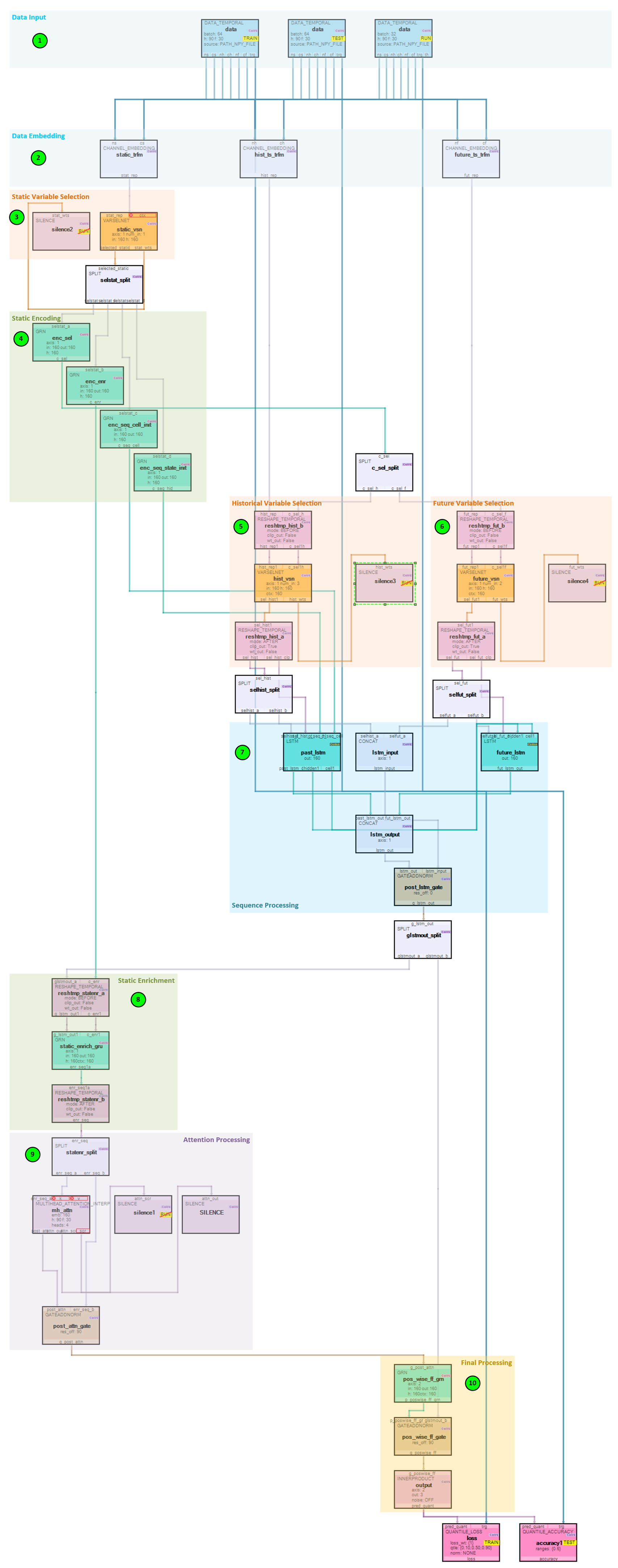
However, if we look at each step the model takes, you will see the magic of this model.
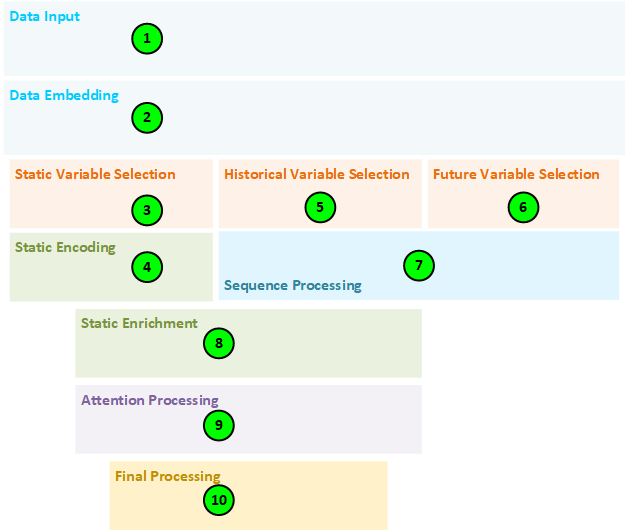
The following describes the step-by-step processing taken by the model.
- The Data Temporal layers in the model are responsible for collecting batches of data for each of the train, test and run (validation) phases of the model. During each phase, the three classes of data are loaded: static non-time dependent data (such as a store location or product number); observed data that includes data only available up to the present (e.g., a stock price, or number of product units sold); and known data that is known both in the past and future (e.g., holiday dates and other date and time related data). There are two types of data in each of these classes of data: numerical data (such as a stock price) and categorical data (such as a stock symbol from a set of stock symbols). The Data Temporal layers organize their outputs into static, historical, and future data where the static data flows into the static, the observed and past known data are combined for the historical data, and the future known data is output as the future data.
- The Channel Embedding layers create embeddings for each of the static, historical and future data by running each numerical variable through an individual Inner Product (linear) projection layer and each categorical variable through an Embed layer.
- The static embeddings are run through a Variable Selection Network (VSN) layer designed to learn the impact each static variable has on the final predictions. The VSN weights are later used when analyzing and visualizing the amount of impact each variable made on the predictions.
- The static VSN outputs are fed into a set of Gated Residual Network (GRN) layers, which “enable efficient information flow with skip connections and gating layers.” [1] The static GRN’s produce the static c_selection fed into the Historical and Future VSN’s; the static c_enrichment fed into the static enrichment GRN; and the c_cell and c_hidden static inputs fed into the first LSTM layer used during sequential processing.
- The historical embeddings are run through a Variable Selection Network (VSN) designed to learn the impact each historical variable has on the final predictions. The VSN weights are used later when analyzing and visualizing the amount of impact each variable made on the predictions.
- The future embeddings are run through a Variable Selection Network (VSN) designed to learn the impact each future variable has on the final predictions. The VSN weights are used later when analyzing and visualizing the amount of impact each variable made on the predictions.
- The outputs of the Historical and Future VSN’s are fed into a set of LSTM layers where the first LSTM acts as an encoder and the second a decoder. The historical VSN output is fed into the encoder LSTM layer and the future VSN output is fed into the decoder LSTM layer.
- The outputs of the historical and future LSTMs are combined and sent to the static enrichment GRN to enhance the temporal features, for “static covariates often have a significant influence on the temporal dynamics (e.g., genetic information on disease risk).” [1]
- The outputs from the static enrichment step are fed into an Interpretable Multi-Head Attention layer which performs self-attention “to learn long-term relationships across different time-steps” [1].
- During the final processing, the self-attention layer outputs are feed through a GRN, normalized in a GateAddNorm layer and passed to a final Inner Product (linear) layer that output the predicted quantiles over the future time steps. When training, these predictions are fed into the Quantile Loss layer and when testing they are fed into the Quantile Accuracy layer.
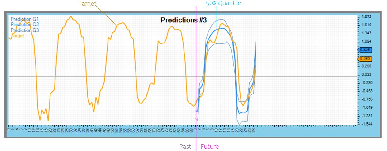
The final predictions comprise a set of desired quantiles (e.g., 10%, 50% and 90%) where the 50% should closely predict the target with the 10% and 90% representing the predicted outer bounds.
Analyzing Model Results
Not only does this model provide powerful predictions, but it does so in a way that allows for easy post training analysis to see how each input variable contributed to the predicted results. Each Variable Selection Network layer outputs a set of weights that show the contributions of each variable.
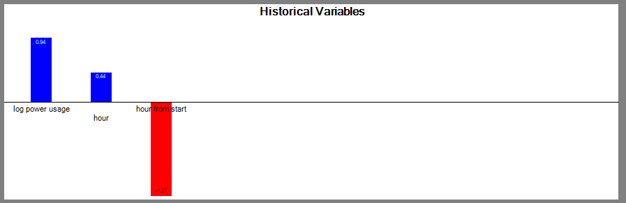
For example, the variables above are from the TFT model used to predict electricity usage and show that the log power usage variable contributed most out of the historical variables to the prediction followed by the hour of the day.
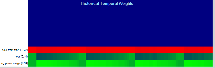
By analyzing the contributions temporally (over time), we can also see that the contributions pick up cycles within the data.
The Interpretable Multi-Headed Attention layer outputs the attention scores which reveal where the attention is focused.
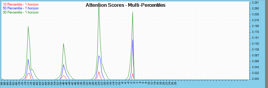
By analyzing the attention scores across percentiles, we can also see a 24-hour periodic pattern in the data.
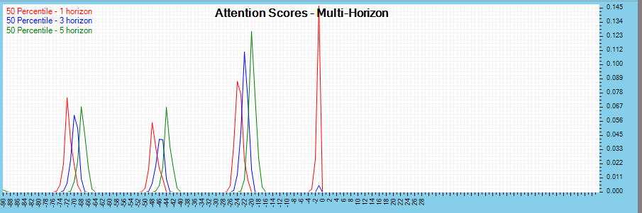
The attention scores can also be analyzed across multiple time horizons for further analysis.
For more information on using the Temporal Fusion Transformer to predict electricity usage, see the TFT Electricity Tutorial. And to see how Temporal Fusion Transformers can predict traffic flow, see the TFT Traffic Tutorial.
New Features
The following new features have been added to this release.
- CUDA 11.8.0.522/cuDNN 8.8.0.121/nvapi 515/driver 516.94
- Windows 11 22H2
- Windows 10 22H2, OS Build 19045.2604, SDK 10.0.19041.0
- Upgraded to Google ProtoBuf 3.23.2
- Added phase selection to Weight visualization.
- Added Temporal Fusion Transformer support.
- Added a new TFT Electricity Dataset Creator.
- Added a new TFT Traffic Dataset Creator.
- Added TFT Analytics with Test Many.
- Added new DataTemporal Layer.
- Added new ChannelEmbedding Layer.
- Added new VarSelNet Layer.
- Added new GRN Layer.
- Added new GateAddNorm Layer.
- Added new ReshapeTemporal Layer.
- Added new MultiHeadAttentionInterp Layer.
- Added new QuantileLoss Layer.
- Added new QuantileAccuracy Layer.
Bug Fixes
The following bug fixes have been made in this release.
- Fixed bug, added save images support to results.
- Fixed bug, now allow empty extension to FILETYPE in properties.
- Fixed bug, import VGG16 onnx, now doesn’t default to detection.
- Fixed bug, force test now outputs status correctly.
- Fixed bug, dialog noted when applying SSD annotations where none exist.
For other great examples, including using Single Shot Multi-Box to detect gas leaks, or using Neural Style Transfer to create innovative and unique art, or creating Shakespeare sonnets with a CharNet, or beating PONG with Reinforcement Learning, check out the Examples page.
Happy Deep Learning with MyCaffe!
[1] Temporal Fusion Transformers for Interpretable Multi-horizon Time Series Forecasting, by Bryan Lim, Sercan O. Arik, Nicolas Loeff, and Tomas Pfister, 2019, arXiv:1912.09363
[2] GitHub: PlaytikaOSS/tft-torch, by Playtika Research, 2021, GitHub