

In our last post, we looked at the organization of the data used by Temporal Fusion Transformer models as described in the Temporal Fusion Transformers for Interpretable Multi-horizon Time Series Forecasting article by Lim et al. [1].
In this post we take a deeper dive into the architecture of the Temporal Fusion Transformer model and how data flows through it – based on the Python implementation in [2] [3].
The Temporal Fusion Transformer model is a complicated model that combines LSTM and self-attention to learn how to predict unknown future time series data points from known past and known future data (e.g., dates, holidays, etc.) The following shows how the data flows through the model from the input batch to the predicted quantiles.
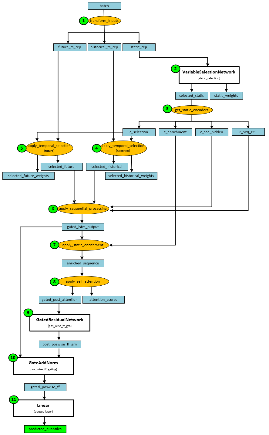
During the forward pass, the following steps take place.
- In the first step, the batch of data is converted into the future, historical and static representations.
- The static representation is then fed into a VariableSelectionNetwork for static selection.
- The static selection output is used to get the static encoders which produce the selection, enrichment, sequence hidden and sequence cell.
- Temporal selection is applied to the historical representation along with the static selection to produce the selected historical data.
- Temporal selection is also applied to the future representation along with the static selection to produce the selected future data.
- Sequential processing is applied to the future and historical selected data to produce the gated LSTM output.
- Static enrichment is applied to the gated LSTM output to produce the enriched sequence.
- Self-attention is applied to the enriched sequence to produce the gated post attention and attention scores.
- The gated post attention is run through a GatedResidualNetwork to produce the postwise grn data.
- The postwise grn data is run through a GateAddNorm layer to produce the gated postwise data.
- The gated postwise data is run through a final Linear layer to produce the predicted quantiles.
Let’s now example each of the sub-sections in detail.
Step 1 – Transforming Inputs
Each batch received is transformed into the future, historical and static representations.
When transforming the inputs, the batch data is transformed into the future, historical and static representations with the following steps.
- The ‘future_ts_numeric’ and ‘future_ts_categorical’ items are pulled from the batch and run through the future_ts_transform InputChannelEmbedding layer to produce the future embedding.
- The ‘historical_ts_nueric’ and ‘historical_ts_categorical’ items are pulled from the batch and run through the historical_ts_transform InputChannelEmbedding layer to produce the historical embedding.
- The ‘static_feats_numeric’ and ‘static_feats_categorical’ items are pulled from the batch and run through the static_transform InputChannelEmbedding layer to produce the static embedding.
In step 2 the static representation is passed through a VariableSelectionNetwork to produce the selected static output.
Step 3 – Get Static Encoders
The static encoders are intended to “yield signals which are designed to allow better integration of the information from static metadata.” [3]
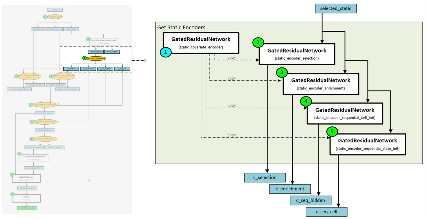
The following steps occur when getting the static encoders.
- During the initialization step, the GatedResidualNetwork ‘static_covariate_encoder’ is copied to each of the four GatedResidualNetworks used to encode the selection, enrichment, sequence hidden and sequence cell data.
- The selected static data is run through the GatedResidualNetwork for static encoder selection to produce the selection embedding.
- The selected static data is run through the GatedResidualNetwork for static encoder enrichment to produce the enrichment embedding.
- The selected static data is run through the GatedResidualNetwork for static encoder sequential cell to produce the sequence hidden embedding.
- The selected static data is run through the GatedResidualNetwork for static encoder sequential state to produce the sequence cell embedding.
Step 4 – Apply Temporal Selection to Historical Data
The temporal selection is applied to the historical embedding to produce the selected historical data.
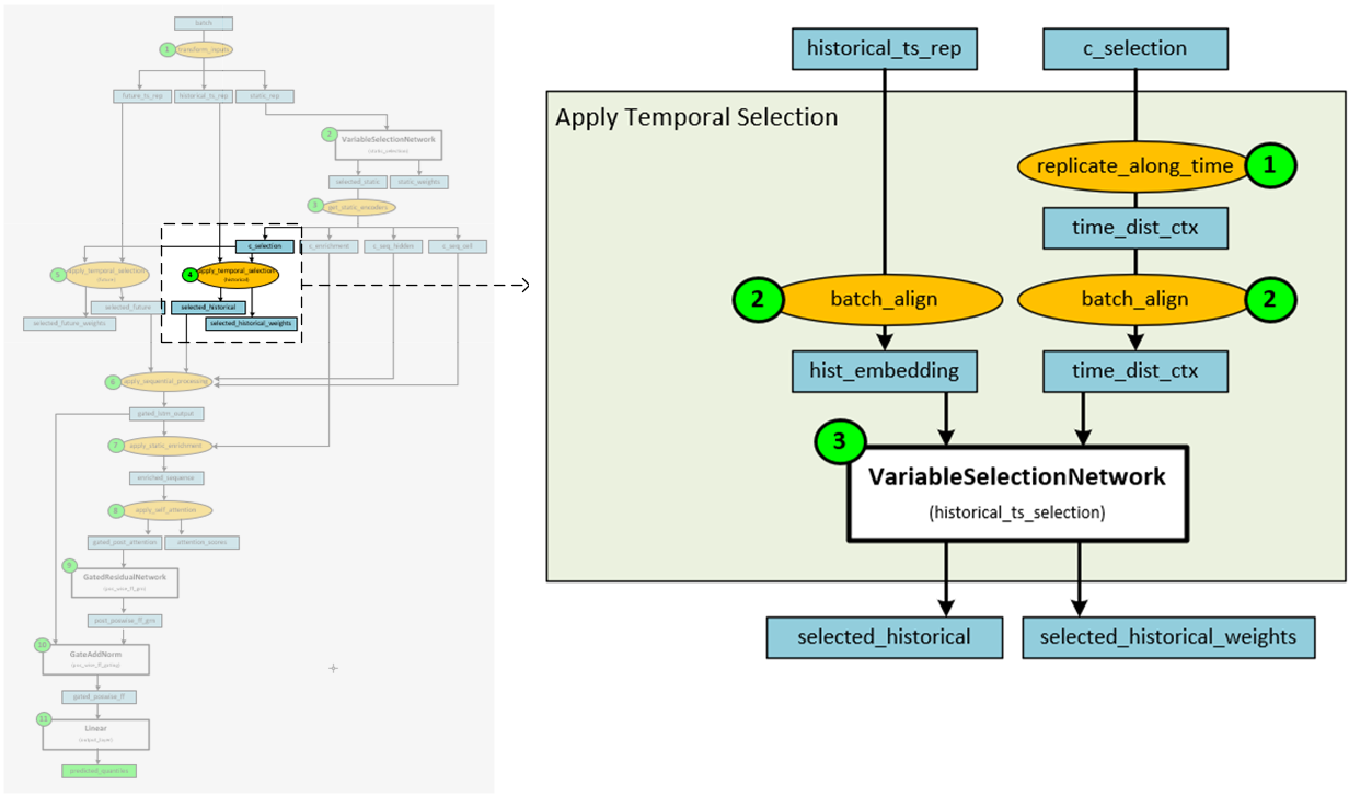
The following steps occur when applying the temporal selection to the historical embedding.
- First the static data is replicated across time.
- Next the static and historical data are aligned to the batch along the same axis.
- The aligned static and historical data are then fed into a VariableSelectionNetwork to produce the selected historical data.
Step 5 – Apply Temporal Selection to Future Data
The temporal selection is applied to the historical embedding to produce the selected future data.
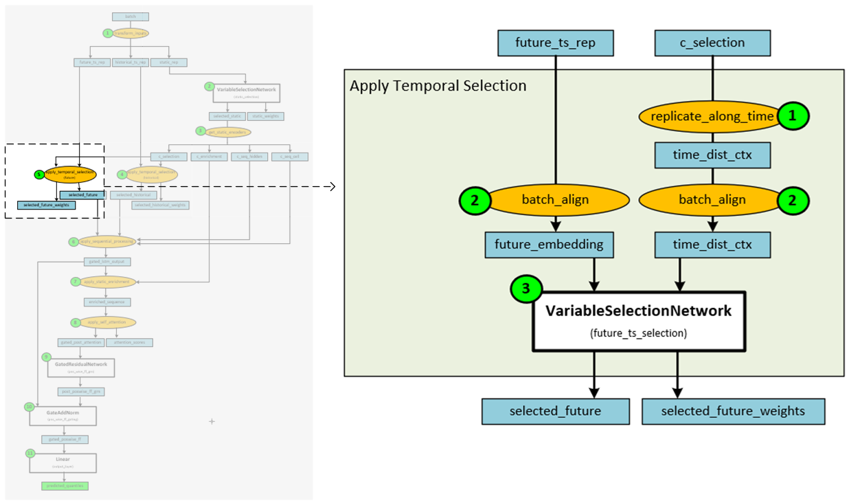
The following steps occur when applying the temporal selection to the future embedding.
- First the static data is replicated across time.
- Next the static and future data are aligned to the batch along the same axis.
- The aligned static and future data are then fed into a VariableSelectionNetwork to produce the selected future data.
Step 6 – Apply Sequential Processing
Sequential processing is applied to the selected historical and future data in such a way that mimics a sequence-to-sequence layer where the historical data is fed into the encoder and the future data is fed into the decoder. “This will generate a set of uniform temporal features which will serve as inputs into the temporal fusion decoder itself.” [3]
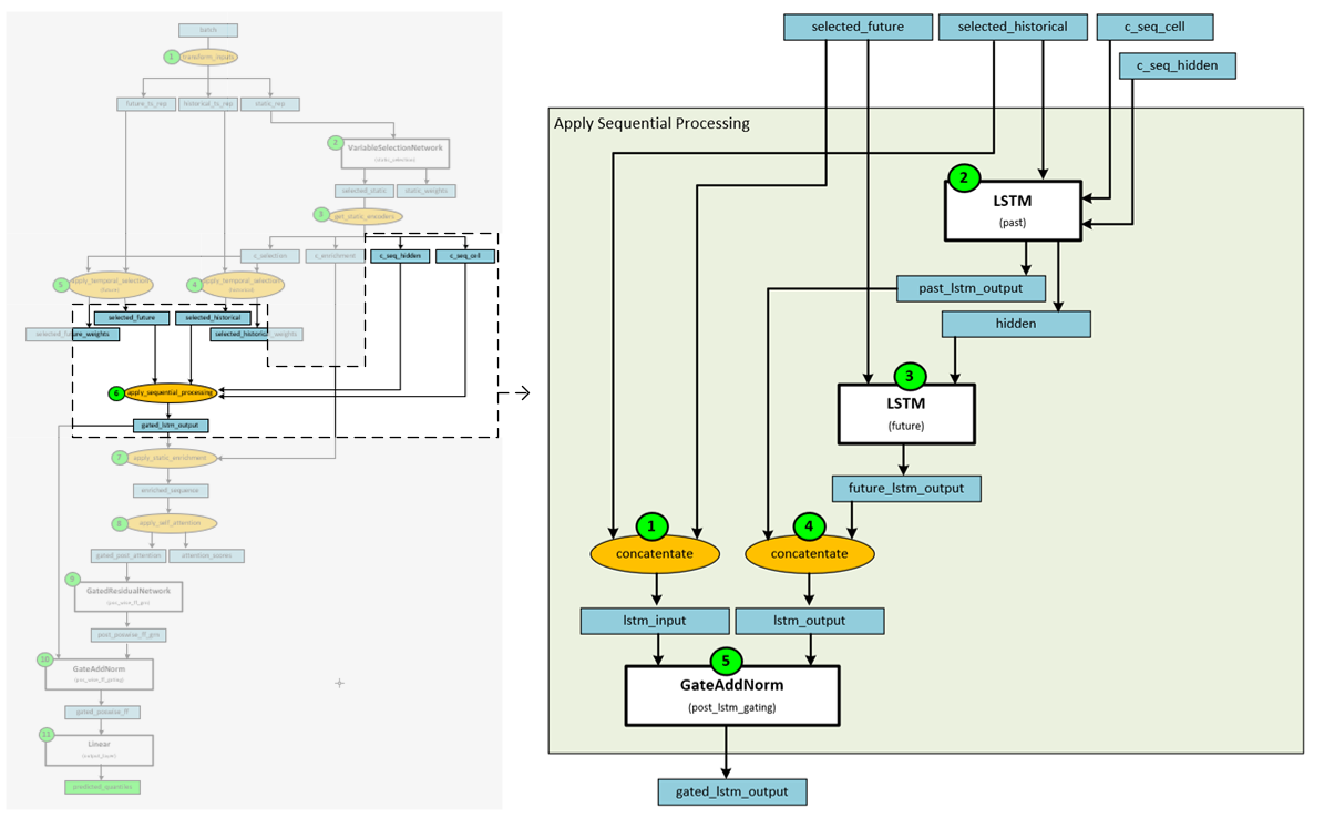
The following steps occur when applying the sequential processing.
- First the selected historical and selected future data are concatenated to produce the lstm input data.
- The selected historical data and sequential cell and sequential hidden data are fed into the first ‘past’ LSTM layer. “To allow static metadata to influence the local processing, we use ‘c_seq_hidden’ and ‘c_seq_cell’ context vectors from the static covariate encoders to initialize the hidden state and cell state respectively.” [3]
- The selected future data and hidden output of the first LSTM layer are fed into the second LSTM layer to produce the future lstm output.
- The past lstm output from the first LSTM layer and the future lstm output from the second LSTM layer are concatenated to produce the lstm output data.
- The lstm input and lstm output data are fed into a GateAndNorm layer to produce the gated lstm output.
Step 7 – Apply Static Enrichment
Static enrichment is applied to the gated lstm output to produce an enriched sequence that is “enhanced [with] temporal features [from] static metadata.” [3]
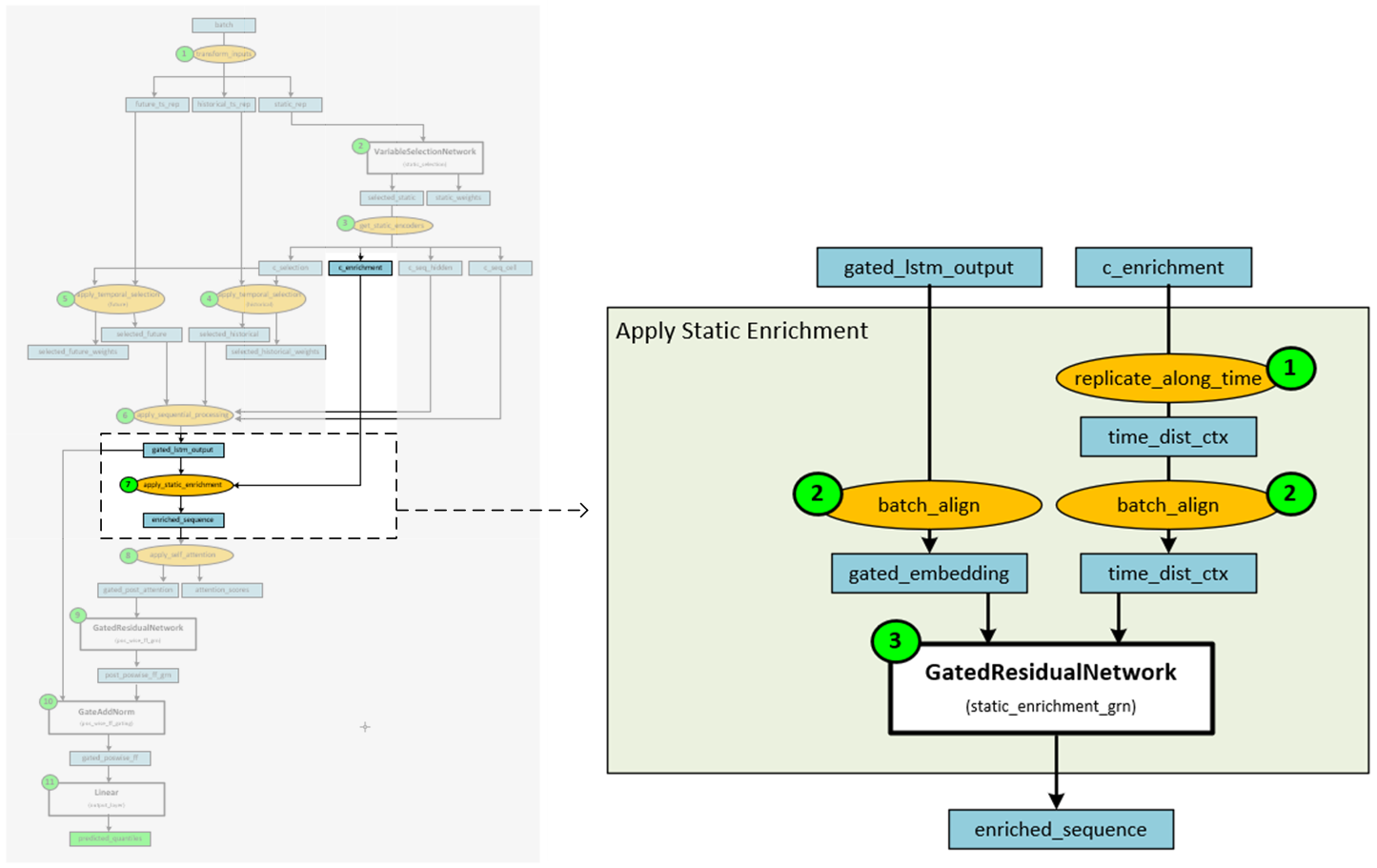
When applying static enrichment, the following steps take place.
- First the static enrichment data is replicated across time.
- Next, the static enrichment and gated lstm data are aligned to the batch along the same axis.
- The aligned static enrichment and gated lstm data are then fed into a GatedResidualNetwork to produce the enriched sequence.
Step 8 – Apply Self Attention
Self-attention is applied to the enriched sequence data to produce the gated post attention data and attention scores. This step can help the model focus on the most important features within the data.
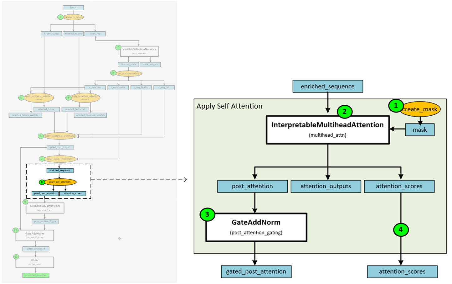
The following steps occur when applying self-attention.
- The attention mask is created to avoid peeking into the future.
- The enriched sequence data and mask are fed into the InterpretableMultiheadAttention layer to produce the post attention, attention outputs and attention scores.
- The post attention data is fed into a GateAndNorm layer to produce the gated post attention data.
- The attention scores are returned along with the gated post attention data.
After applying the attention, the network continues with step 9 where the gated post attention data is sent through a GatedResidualNetwork layer, then GateAddNorm layer to produce the postwise grn data. In step 10, the gated lstm output is added to the postiwise grn data via a GateAddNorm layer which produced the gated postwise data. And in the final step 11, the postwise gated data is fed into a Linear layer to produce the predicted quantiles.
And that concludes the data flow through the Temporal Fusion Transformer model from batch to predicted quantiles.
Happy Deep Learning!
[1] Temporal Fusion Transformers for Interpretable Multi-horizon Time Series Forecasting by Bryan Lim, Sercan O. Arik, Nicolas Loeff and Tomas Pfister, 2019, arXiv:1912.09363
[2] GitHub: PlaytikaOSS/tft-torch by Dvir Ben Or (Playtika), 2021, GitHub
[3] GitHub: PlaytikaOSS/tft-torch Training Example by Dvir Ben Or (Playtika), 2021, GitHub