

ChatGPT is an amazing technology that has taken the world by storm. Under the hood, a highly trained large language model (LLM) creates the response to each query sent to the service. In February 2023 Meta released the open-source Llama2 LLM and on September 29, 2023, Meta released an open-source Llama2-Long LLM [1] which appears to rival ChatGPT’s internal private LLM models by using a Rotary Position Encoding (RoPE) [2]. Now, anyone can download and run the Llama2 models for free.

Chat Process (used by Llama2.c and ChatGPT type models)
By now anyone who has used ChatGPT is familiar with the general process. You type in a system prompt followed by a user prompt and then start a conversation with the system using an underlying LLM. Running the Llama2.c application is no different and uses the following process.
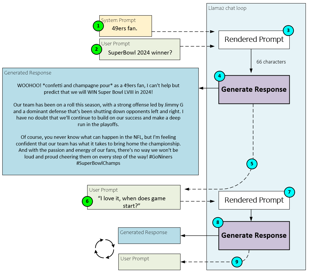
When using the Llama2.c application, the following steps occur.
- The user (optionally) types in a system prompt, such as
“49ers fan.”
- Next the user types in the user prompt, such as
“SuperBowl 2024 winner?”
- These two prompts are fed into the Llama2 application which constructs the model input rendered prompt which usually contains additional internal chat instructions such as ‘INST’ for instruction and ‘SYS’ for system prompt.
- The rendered prompt is fed to the internal LLM processing (discussed in detail later) which generates the response,
“WOOHOO! *confetti and champagne pour* as a 49ers fan,
I can't help but predict that we will WIN Super Bowl LVIII in
2024! Our team has been on a roll this season, with a strong
offense led by Jimmy G and a dominant defense that's been
shutting down opponents left and right. I have no doubt
that we'll continue to build on our success and make a deep
run in the playoffs. Of course, you never know what can
happen in the NFL, but I'm feeling confident that our team
has what it takes to bring home the championship. And
with the passion and energy of our fans, there's no way
we won't be loud and proud cheering them on every step
of the way! #GoNiners #SuperBowlChamps”
The first thing any 49’ers fan will notice is that the 49ers are no longer led by Jimmy G. as he departed the team after the 2022 season. The main reason for this is that Llama2, like other current LLM’s, only stores knowledge up until the model was last trained, which must have been sometime before Jimmy G. left the team. As a side note, this is why technologies such as LoRA are exciting, for they provide an efficient manner to fine-tune large language models with more updated information.
- After the prompt response is returned, the user is asked for another prompt.
- This time, the user enters a prompt, but without a system prompt.
- The user prompt is then rendered internally to include the ‘INST’ instruction.
- Next, the rendered prompt is processed to generate the response that is returned to the user.
- The user is asked for another prompt and the cycle continues back at step #6 above.
Chat Process Internals
Internal to the Llama2 application, there are three main objects that work together to digest the user prompts and generate the response. These are the Tokenizer, Transformer and Sampler.
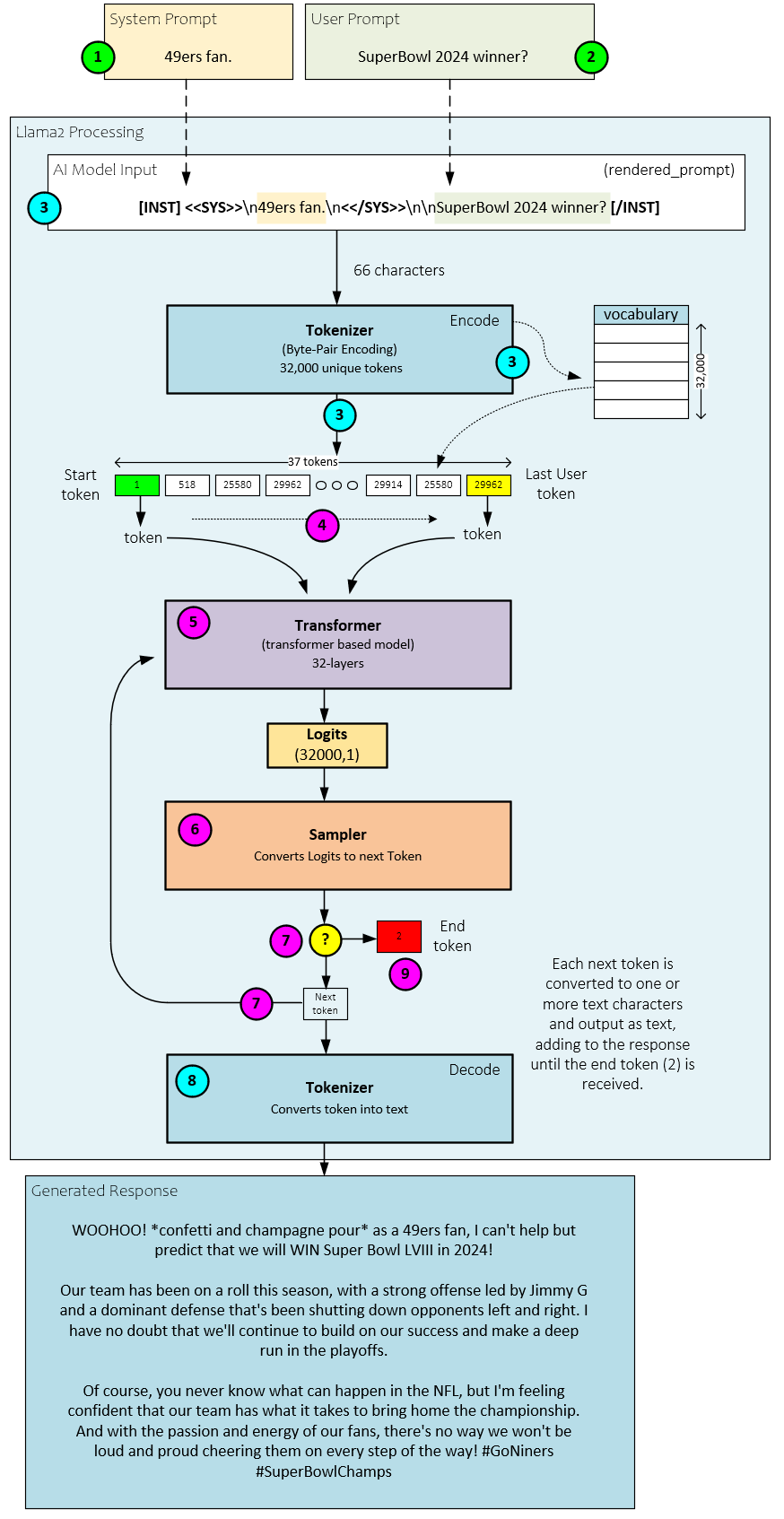
The Tokenizer is responsible for converting the input text rendered prompt into a sequence of numbers called tokens. Each number is a numeric index into the large language models vocabulary. The vocabulary stores all characters and sub-words used by the language supported by the model – the Llama2 model has a vocabulary of 32,000 unique tokens.
The Transformer is responsible for running the tokens through the trained weights, where the weights store the learned knowledge of the model. Each token, yes token by token, is run through the model one at a time. A vector of numbers called logits is output by the Transformer for each token processed. Each entry in the logits vector represents one of the 32,000 vocabulary token slots.
The Sampler is responsible for converting the logits back to tokens using either a greedy arg-max function or a probability-based sampling method. After processing each token of the input, the token output by the Sampler is then fed back into the Transformer as the input used to generate the next token. This process continues until the end token is reached. At each step, the token output by the Sampler is also decoded back into its text representation and output to the user.
The following is a more detailed set of steps that occur during this process.
- The user types in the system prompt.
- Next the user types in the user prompt.
- The system and user prompts are combined into the rendered prompt that is sent to the Tokenizer which converts the rendered prompt into the input tokens using the Byte-Pair Encoding algorithm [4].
- Each input token is fed into the Transformer starting with the start token.
- The Transformer Forward method processes each token in turn by running the token at the current position through each of its layers (e.g., 32 layers in the 7B parameter Llama2 model). Each pass through the Forward method produces a vector of 32000 numbers called logits where each logit corresponds to one of the 32,000 slots within the language vocabulary.
- The logits are passed to the Sampler which converts the logits to the next token value. For example, the 32,000-item vector is converted into the appropriate next token numerical value (more on this process later).
- If the original token was an input token, then the process continues at step #4 with the next input token. After all input tokens are processed and the next token is the end token, the output generation stops, and the user is asked for another prompt. If all input tokens are processed and the next token is not an end token, the next token is passed back to the Transformer and used as the next input token in step #5 above.
- After processing all input tokens in this cycle, each new token produced is also decoded by the Tokenizer to convert the token back to its text representation which is output to the user. After the decoded text is output to the user the process continues at step #5 above until the end token is reached.
- Once the end token is reached, the output generation process stops, and the user is asked for a new prompt.
Next let us look at each of these steps in more detail starting with the Tokenizer encoding process.
Tokenizer Encoder
The Tokenizer encodes each character in the rendered prompt into a set of input tokens using the vocabulary loaded during the initialization process along with the Byte-Pair Encoding (BPE) algorithm [4].
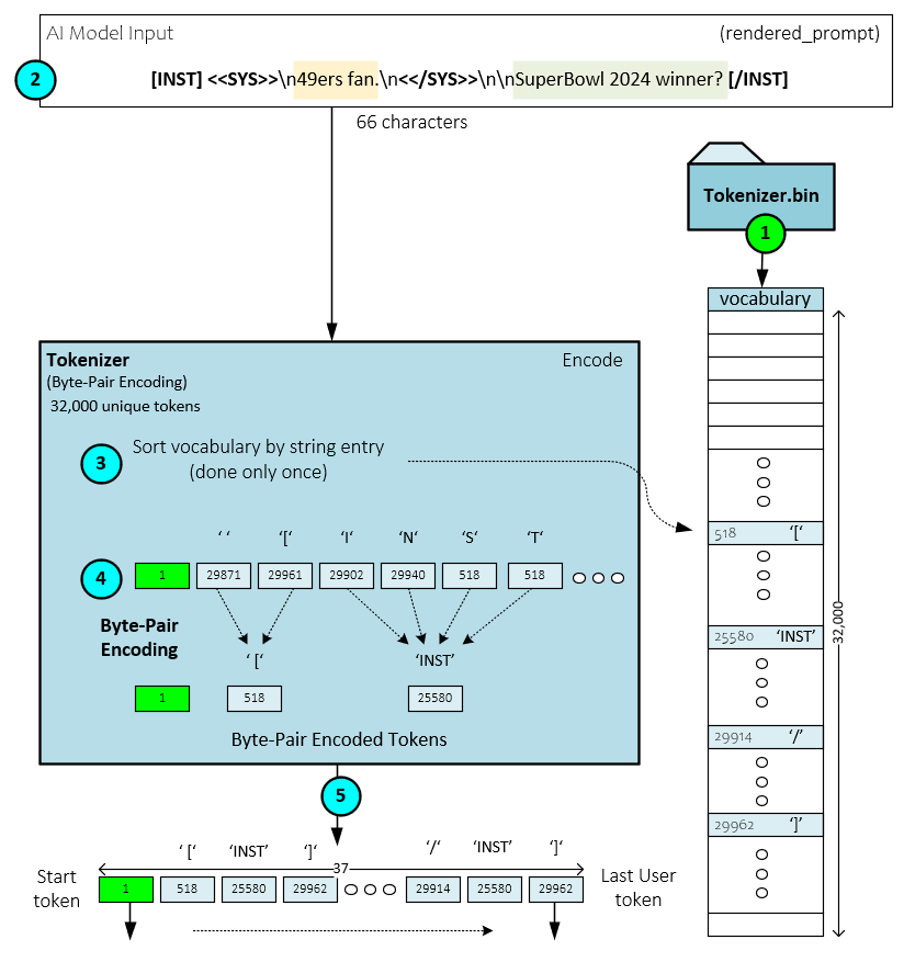
The following steps occur during the token encoding process.
- During initialization, the Tokenizer loads the Byte-Pair Encoding vocabulary from the bin file. The BPE algorithm is a compression algorithm used to describe text in a more compact form than its original form. The BPE algorithm is a popular sub-word tokenization algorithm used by many LLM’s such as GPT-2, RoBERTa, XLM, FlauBERT and Llama2. [5]
- When processing prompts, the rendered text prompt is sent to the Tokenizer.
- Internally, the Tokenizer first sorts the vocabulary by its string entries – this is only done once to make token lookup faster.
- Each character of the input rendered prompt is first converted to its corresponding character token and then combined using the BPE algorithm until all pairs are accounted for.
- The ‘compressed’ set of tokens is returned as the set of input tokens. For example, our 66 characters of rendered prompt text is compressed down to a total of 37 input tokens.
Transformer Processing
Given the Transformer complexity, we will describe its processing in stages, stating with a summary of what it does.
The main goal of the Transformer is to process each token (one at a time, starting with the start token) and produce the logits corresponding with each, where the logits for a token is a 32,000-item vector of numbers that correspond to each of the slots in the vocabulary. During this conversion process, the following steps take place.
- First, tokens are fed one at a time through the Transformer’s Forward method where the following steps take place per token.
- Given a token, a vector of size dim is copied from the token embedding values associated with the token location (in the vocabulary) to the x Tensor. The embedding values are part of the checkpoint weight file loaded during the build process (discussed later).
- Next, the x Tensor is fed into the layer processing where each of the 32 layers process the values in sequence starting with normalization, scaling by the rms_att weights, and processing the QKV projections.
- The RoPE [2] positional information is added to the q and k Tensors and the k and v Tensors are cached.
- Attention processing is performed on the q, k, and v Tensors along with the k and v Tensor Keep in mind that this is where the main knowledge of the model is applied.
- The attention processing result is added to the x Tensor as a residual.
- Next, the w1, w2, w3 weights are used along with the SwiGLU activation for the ffn
- The ffn outputs are then added to the x Tensor as a residual. The resulting x Tensor is passed back to the start of step #3 for the next layer’s processing. This cycle from step #3-8 continues until all 32 layers have processed the data.
- Upon completion of the last layer of processing, the final processing starts with the following sub-steps.
- The x Tensor is normalized and scaled by the rms_final weights with the results paced in the xb Tensor.
- The normalized and scaled xb Tensor is quantized, …
- …, and a MatMul is performed between the quantized xb values and the wcls weights (which were already quantized during the build step), to produce the final logits Tensor.
The final logits Tensor (which corresponds to the input token) is returned.
Transformer Processing – Digging Deeper
If you are uninterested in all the details of the Transformer Processing, feel free to skip to the Sampler section. Before Transformer processing begins, the Transformer must be built using the Build method.
Building The Transformer
Large language models are, well large. Depending on the quantization of the Llama2 model, the model weight files range from 7GB (8-bit quantization) up to 26GB (no quantization). For this reason, the Llama2 application uses a memory mapped file where the actual weight values are not directly loaded, but instead pointers are used by each of the Tensor and QuantizedTensor objects to point directly to the weights in the memory mapped file. The loading and setting up of these tensors occur within the Build method called during initialization.
During the building process, the following steps occur.
- First, just configuration information the header of the bin file (e.g., the 7B parameter weight file) is read. Keep in mind the checkpoint.bin file uses a unique, program agnostic format unique to the Karpathy’s llama2.c program. In other words, this file format is not PyTorch specific like the PTH files usually used to store model weights. After reading the header information a memory mapped file is created and used to set the pointer values for all other weights.
- The Config object containing the hyperparameters is initialized with the configuration information.
- QuantizedTensor and Tensor objects store the pointers to the weight values.
- QuantizedTensor and Tensor objects also holds a pointer to the Primitives object used for low-level CPU or GPU operations.
- QuantizedTensor and Tensor objects exist for each of the weights including the wq, wk, wv, wo, w1, w2, and w3 weights for each layer.
- Next, the RunState is created containing all non-weight tensors used when running through the layer processing and final processing of each Forward pass.
Once built, the Transformer is ready to process tokens via its Forward method.
Transformer Processing – In Detail
The following sections describe specific details of the Transformer Forward pass.
Pre-Layer Processing
Pre-layer processing involves copying the embedding for the current token into the x Tensor.
During pre-layer processing, the following steps occur.
- First, tokens are fed one at a time through the Transformer’s Forward method where each of the following steps take place for each token.
- Given a token, the token embedding, a vector of size dim, is copied into the x Token. The embedding values are loaded during the build process and are part of the weight file.
Normalize, Scaling and QKV Projections
Step #3 is the start of the layer processing loop that runs from step #3-8 sequentially through each of the 32 layers (for the 7B parameter model). During this step, the x Tensor is normalized, scaled by the rms_att weights, and used to create the q, k, and v projections.
During the normalization, scaling and QKV projections the following steps occur.
3.a) The x Tensor is normalized and scaled using the rms_att weights where the normalization is like a LayerNorm operation, and the results are then scaled by multiplying with the rms_att weights.
3.b) Next, the normalized, scaled results are quantized into the xq QuantizedTensor.
3.c) A MatMul operation is performed between the xq QuantizedTensor and each of the wq, wk, wv weights that are already quantized. These three operations produce the q, k, and v Tensor projections.
Adding RoPE Positional Information
RoPE positional information is applied to the q and k Tensors as this positional information helps the attention process. “RoPE enables valuable properties, including the flexibility of sequence length, decaying inter-token dependency with increasing relative distances, and the capability of equipping the linear self-attention with relative position encoding.” [2] Additionally, the k and v Tensors are cached at this stage.
The following steps occur when adding RoPE and caching.
4.a) The RoPE primitive is used to add the position information to both the q and v Tensors.
4.b) Next, the k Tensor is cached in the key_cache.
4.c.) Next, the v Tensor is cached in the value_cache.
We are now ready for the attention processing.
Attention Processing
Attention processing performs self-attention using the q, k, v, key_cache, and value_cache Tensors by applying the standard QKV attention function on the values. The attention processing occurs across each of the n_heads for the q, k, v, key_cache and value_cache inputs.
The following steps occur during the attention processing.
5.a) The q, k, v, key_cache, and value_cache Tensors are sent to the CalculateAttention primitive which performs the attention as described by Vaswani et al. [6] to produce the xb Tensor.
5.b) The attention xb Tensor outputs are then quantized.
5.c) A MatMul operation is performed between the quantized xb values and the already quantized wo weights to produce the xb2 Tensor outputs.
6.) The xb2 Tensor outputs are added to the x Tensor as residuals.
The CaclulateAttention primitive calculates attention as defined by Vaswani, et. al, [6]. In specific, the attention function below is performed on the q, k, and v Tensors:
![]()
![]()
W1, W2, W2 and Activation
The x Tensor values next move to the w1, w2 and w3 processing with activation.
The following steps occur when processing the W1,2,3 weights with activation.
7.a) The x Tensor is normalized with the RmsNorm operation and the rms_ffn weights and the results are placed in the xb Tensor.
7.b) Next, the xb Tensor is quantized.
7.c) A MatMul operation is performed between the quantized xb values and the already quantized w1 weights and the result is placed in the hb Tensor.
7.d) A MatMul operation is performed between the quantized xb values and the already quantized w3 weights and the result is paced in the hb2 Tensor.
7.e) The hb2 Tensor is run through the SwiGLU activation whereas noted by Shazeer, “The GEGLU and SwiGLU variants [of GLU] produce the best perplexities.” [8] Note, the SwiGLU operation internally uses both the hb and hb2 values in its calculation and places the results back into the hb Tensor.
7.f) Next, the hb Tensor is quantized.
7.g) And a MatMul operation is performed between the quantized hb values and the already quantized w2 weights to produce the new hb2 Tensor values.
8.) The new hb2 Tensor values are added to the x Tensor as residuals. If there are more layers to process, the x Tensor becomes the new input to the new layer and the processing starts again at step #3 above. Otherwise, final processing occurs next.
Final Processing
In the final processing, another normalization and scaling occur followed by a final MatMul to produce the final logits for the token being processed.
The following steps occur during final processing.
9.a) The x Tensor is normalized and scaled by the rms_final weights and paced in the xb Tensor.
9.b) Next, the normalized and scaled xb Tensor is quantized, …
9.c) …, and a MatMul is performed between the quantized xb values and the wcls weights (which were already quantized during the build step), to produce the final logits Tensor.
And that concludes the full processing taking place during the Forward pass of the Transformer. Keep in mind that all this processing occurs for each token.
Click on the image below for the full Transformer Forward pass.
Sampler Processing
The Sampler converts the logits output by the Transformer Forward pass, into the next token numeric value.
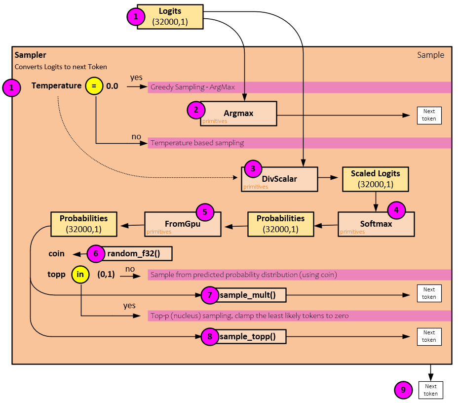
When converting the logits to a token numeric value, the following steps occur.
First the logits output from the Transformer Forward pass is passed to the Sampler and depending on the Temperature value the sampling method is chosen.
- If the Temperature is equal to 0.0, a simple ArgMax operation is performed to select the next token using a greedy sampling.
- Otherwise, the sampling proceeds to the probability-based sampling methods. In preparation for the probability-based sampling, the Temperature is used to scale the logits by dividing the logits by the Temperature According to Renze, et. al., “Despite anecdotal reports to the contrary, our empirical results indicate that changes in temperature in the range 0.0 to 1.0 do not have a statistically significant impact on LLM performance for problem-solving tasks.” [9] However, this hyperparameter controls the randomness of the model outputs where “a lower temperature makes the output of the LLM more deterministic, thus favoring the most likely predictions.” [9]
- The scaled_logits Tensor is run through the Softmax operation to convert the logits to probabilities that sum to 1.0.
- If using a GPU, the probability Tensor is transferred from the GPU to the CPU memory.
- A random value is calculated as the coin (as in a flip of a coin).
- Next if the topp <= 0.0 or topp >= 1.0 then the sampling occurs on the probability distribution via the sample_mult() function which returns the next token numeric value.
- Otherwise, if the topp is within the range (0.0, 1.0) then the Top-p (nucleus) sampling is used which clamps the least likely tokens to zero. This sampling occurs using the sample_topp() function which returns the next token numeric value.
If the next token value is the stop token, the current prompt response ends, otherwise if all input tokens have already been processed, the next token is Decoded by the Tokenizer to text, output to the user, and then passed back to the next Transformer Forward pass as the new token input.
Summary
In this post, we took a deep dive into how Karpathy’s Llama2 [3] software works. We looked at the Tokenizer, Sampler and extensively at the Transformer to show how they work internally and interact with one another to generate responses to user prompts. This short, elegant program really shows how amazing large language models are. The attention weights in large language models reveals a wealth of information that can be accessed with minimal code. It is impressive how much knowledge is encoded in these weights and how easily it can be extracted!
Happy Deep Learning with LLMs!
[1] Effective Long-Context Scaling of Foundation Models, by Wenhan Xiong, Jingyu Liu, Igor Molybog, Hejia Zhang, Prajjwal Bhargava, Rui Hou, Louis Martin, Rashi Rungta, Karthik Abinav Sankararaman, Barlas Oguz, Madian Khabsa, Han Fang, Yashar Mehdad, Sharan Narang, Kshitiz Malik, Angela Fan, Shruti Bhosale, Sergey Edunov, Mike Lewis, Sinong Wang, and Hao Ma, 2023, arXiv:2309.16039
[2] RoFormer: Enhanced Transformer with Rotary Position Embedding, by Jianlin Su, Yu Lu, Shengfeng Pan, Ahmed Murtadha, Bo Wen, and Yunfeng Liu, 2021, arXiv:2104.09864
[3] GitHub:karpathy/llama2.c, by Andrej Karpathy, 2023, GitHub
[4] Byte-Pair Encoding, Wikipedia
[5] Byte-Pair Encoding: Subword-based tokenization algorithm, by Chetna Khanna, 2021, Medium
[6] Attention Is All You Need, by Ashish Vaswani, Noam Shazeer, Niki Parmar, Jakob Uszkoreit, Llion Jones, Aidan N. Gomez, Lukasz Kaiser, and Illia Polosukhin, 2017, arXiv:1706.03762
[7] FlashAttention: Fast and Memory-Efficient Exact Attention with IO-Awareness, by Tri Dao, Daniel Y. Fu, Stefano Ermon, Atri Rudra, and Christopher Ré, 2022, arXiv:2205.14135
[8] GLU Variants Improve Transformer, by Noam Shazeer, 2020, arXiv:2002.05202
[9] The Effect of Sampling Temperature on Problem Solving in Large Language Models, by Matthew Renze and Erhan Guven, 2024, arXiv:2402.05201