

In this post we explore how to train the Llama2 model using the Baby Llama2 created by Andrej Karpathy [1] which is based on his original minGPT model [2] and has the same basic transformer architecture that other generative AI models use, such as ChatGPT [3]. Generative transformer models employ a stack of transformer blocks which internally retain knowledge using weights that store knowledge learned via the Attention mechanism as described by Vaswani et. al. [4] In general transformer models have the following architecture.
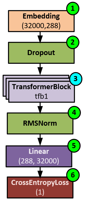
The transformer model is trained to understand natural language input in the form of text that is first tokenized by converting the text to numeric values that are references into a vocabulary dictionary. The tokenized values are used to train the network where the previous tokens predict the next token in the sequence. During the training process, the model first (1) creates an embedding of each token, (2) adds dropout to help the model generalize, and then (3) runs through the stack of 6 to 100+ transformer blocks, each of which contain the attention mechanism used to learn from the inputs. The transformer block results are (4) normalized to keep the model stable, and (5) converted into logits that correspond to each of the vocabulary items, which in this case comprise 32,000 vocabulary items. And finally, during training, (6) the logits are converted back to the predicted ‘next’ token values that are compared with the actual ‘next’ token values using the CrossEntopyLoss to produce the loss value. The loss value is then backpropagated through the network to calculate the gradients that are then applied to the weights using the optimizer thus facilitating the actual learning.
In this post, we will dive deep into the actual data pre-processing, the training process and model data flow occurring during the training.
Pre-Processing
When using Karpathy’s Baby Llama2, the pre-processing occurs in two steps. First the Tiny Stories dataset is downloaded from Hugging Face and extracted. Then the extracted data is converted to tokens in the pre-tokenizing process.
Downloading The Dataset
The Tiny Stories dataset by Eldan et. al. [5] is a collection of short, simple stories created using other versions of GPT, including both GPT 3.5 and GPT 4.0. This dataset is used to train the Baby Llama model from scratch.
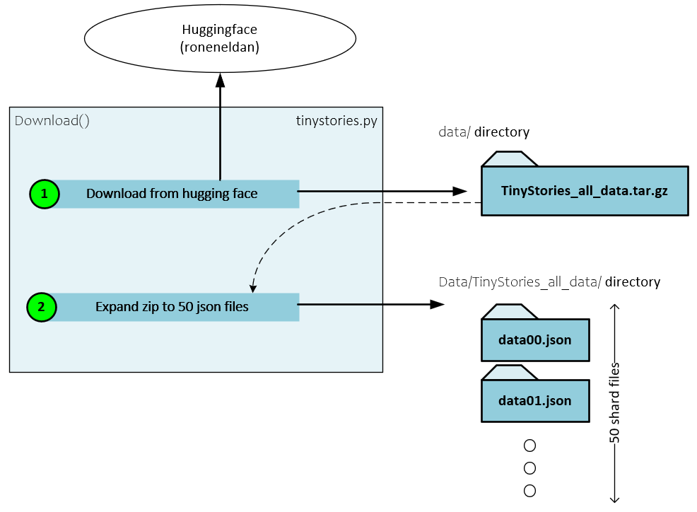
During the downloading process the following steps occur.
- The actual tar.gz raw data file is downloaded to the data directory relative to your Python project.
- Next, the 50 Json data files are extracted from the *.gz file and placed in the data/TinyStories_all_data
Json Data File Content
Each of the 50 Json files contains 100,000 short stories for a total of five million short stories in the entire dataset.
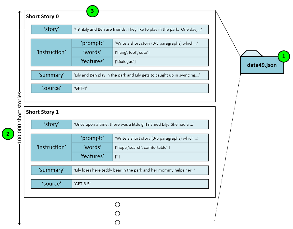
Within a single Json file (1) you will find the 100,000 short stories (2) each stored with the same format (3) containing the following entries as described by [5]:
Story: the story portion contains the actual short story text created using the source model, instructions, and summary.
Instruction: the instruction contains a prompt used to prepare the model, a list of words to be included in the story, and features describing the story’s attributes.
Summary: a summary of the story used to create the actual full story text along with the instructions.
Source: the source is the source model used to create and summarize the short story.
When training the Baby Llama2 model, only the story portion of the data is used.
Pre-Tokenizing The Data
Pre-tokenizing is the process of selecting and converting the raw text into tokens where a token is a numeric index value that references a specific sub-text value within the vocabulary. For example, a 26-character based vocabulary would have twenty-six entries and therefore token values from 0 to 25. As you can imagine, large language model vocabularies are much larger for they consist of not only the characters used but also numerous combinations of the characters used. A common tokenization algorithm used to build a vocabulary is called byte-pair encoding [6] [7]. This type of tokenization method is used by the Llama models, including Baby Llama which builds a vocabulary of 32,000 entries.
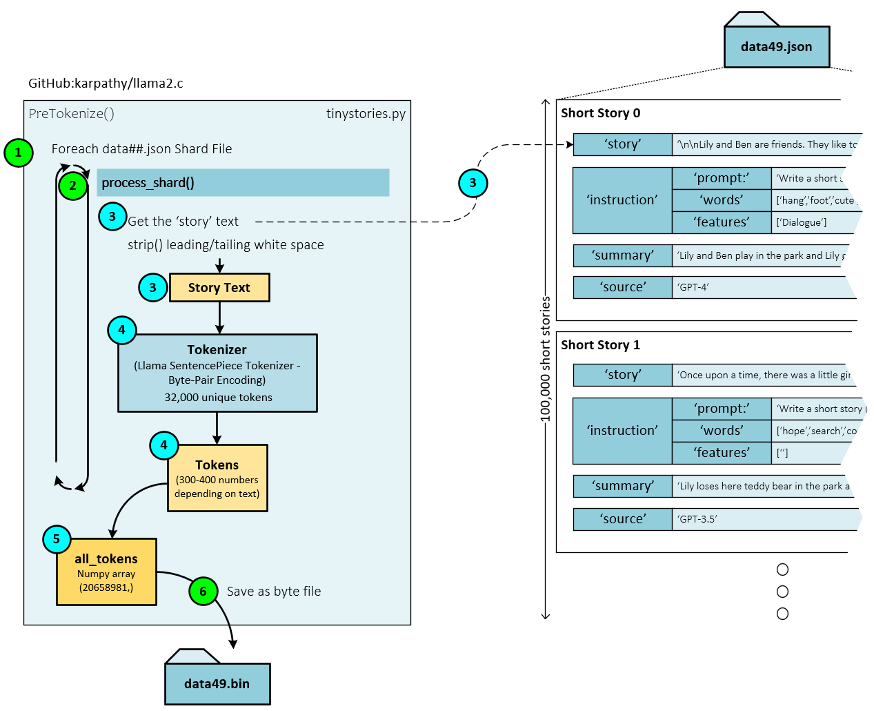
During tokenization, the following steps occur.
- For each Json file (e.g., json), …
- … the process_shard() function tokenizes each of the 100,000 short stories within the Json file.
- During tokenization, first the story text is extracted from the shard.
- Next, the story text is tokenized using the byte-pair tokenization process implemented by the SentencePieceProcessor which is part of SentencePiece.
- The tokens created from each shard are then added to the all_tokens
- Upon completing the tokenization of all shards, the all_tokens list is saved as a byte file to the corresponding data file. For example, the tokenized json shards are saved to the data49.bin binary data file.
Training Model from Scratch
When training from scratch, the model contains randomly initialized weights that have no learned knowledge. The process of training allows the model to learn the knowledge we seek and in the case of the GPT type models such as Llama2 and GPT, the model is trained to predict the next token given a set of input tokens. Keep in mind that input tokens may include the system prompt and user prompt, etc.
During training, the pre-tokenized tokens are used to train the model with the following steps occurring.
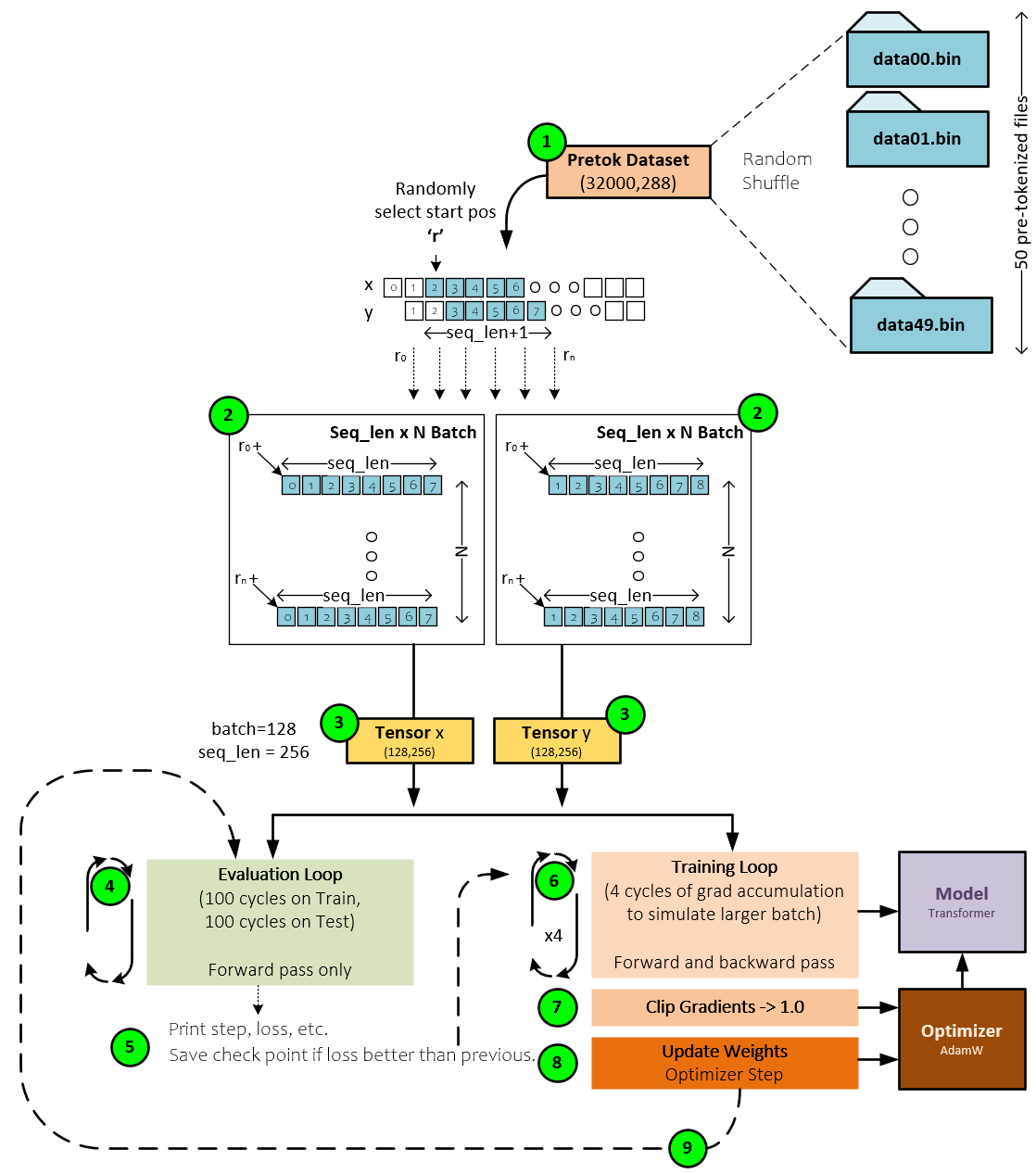
- The Pretoke Dataset loads each pre-tokenized *.bin data file into a memory mapped file that is used when needed and randomly selects the starting point ‘r’ from within the file data. A seq_len of tokens is loaded from the ‘r’ starting point and stored as the current line in the batch being built. Each line of data is seq_len in length. To predict the next token, the Y tensors are offset one token forward in the sequence from that of the X input sequence.
- A grid of token sequences, each of seq_len in length, are stacked to create the X batch, and Y batch where each sequence in the Y batch is shifted by one token forward in corresponding X sequence of tokens.
- The X and Y batches of tokens are placed into Tensors of size (128,256) corresponding to a batch size of 128 and sequence length of 256.
- The X and Y batches are then sent through the evaluation loop that calculates the current training (using the X batch) and testing (using the Y batch) losses. This loop runs for one hundred iterations and the losses calculated are averaged.
- The losses are printed for output and if the test loss is better than the previous loss, the current model check-point weights are saved to disk.
- Next, the training loop is entered to train the model. To simulate a larger batch size, the training loop runs four cycles and accumulates the gradients at each step. These gradients will later be used to alter the model weights which is how the model leans.
- Next, the gradients are clipped to values no larger than 1.0 for model stability.
- And, then the optimizer is used to update the model weights using the learning rate, momentum, weight decay and the optimizer algorithm used. Baby Llama uses the AdamW [8]
- After updating the weights, the training loop continues and at certain iterations re-enters the evaluation loop, or otherwise continues to the next training loop.
Training continues until a sufficiently low and acceptable loss value is observed in the testing dataset that does not diverge from the training loss – which usually indicates overtraining.
Upon completion of the training, the trained weights are the same weights used by the Llama2.c inferencing discussed in our previous blog.
Baby Llama Model
The Baby Llama model is a scaled down version of the same model architecture used by the full Llama2 7B and Llama2 13B models. The main difference between the two models is that the number of layers and model dimensions are much smaller in the Baby Llama model.
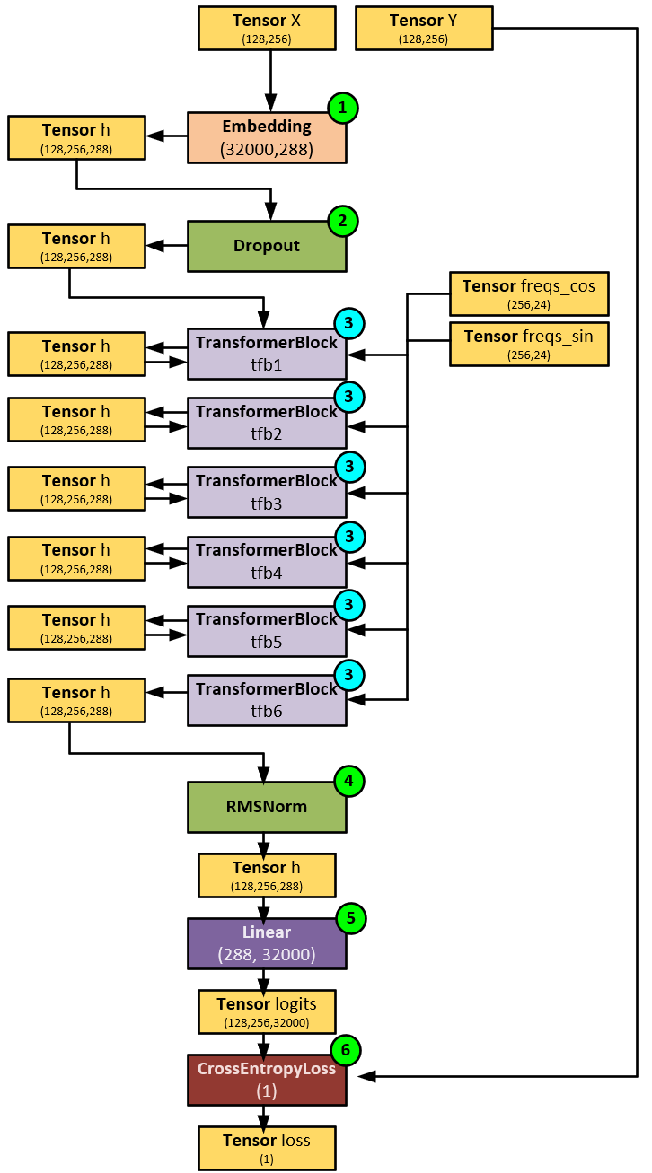
When processing the Baby Llama Model, the following steps occur.
- First, the input batch of tokens in the X tensor of input tokens is sent to the Embedding layer which converts each token into a 288-dimensional embedding. Embeddings are used to spatially separate each of the 32000 potential token values. The output of the embedding process is placed in the h tensor of shape (128, 256, 288) which corresponds to a batch size of 128, sequence length of 256 tokens, each with a dimension of 288 for the embedding. Note, the larger Llama2 models use an embedding size of 4096.
- Next, the h tensor is passed through a Dropout layer to help regularize the model.
- And then the h tensor is run through the stack of TransformerBlock layers that make up the foundation of the overall model. As you will see later, each TransformerBlock contains the attention mechanism as discussed by Vaswani et. al. [4], which is where the main knowledge learning of the model occurs. The main difference between the Baby Llama Model and larger models such as the 7B Llama2 model is that Baby Llama uses 6 TransformerBlocks corresponding to the 6 layers, whereas the 7B Llama2 Model uses 32 TransformerBlocks corresponding to its 32 layers. Also, note at this stage, the freqs_cos and freqs_sin tensors are fed into each TransformerBlock – these two tensors are used to add positional encoding to the Q and V tensors during CausalSelfAttention (discussed later).
- After the last TransformerBlock the h tensor is normalized with the RMSNorm [9] layer for model stability.
- Then the h tensor is processed by a straight Linear layer which converts the h tensor into the logits of shape (128,256,32000) where each of the 32000 values each represent a probability associated with the predicted token to be next within the vocabulary set.
- A CrossEntropyLoss [10] layer is used to calculate the loss which then feed into the backward pass to calculate the gradients that later update the weights to facilitate model learning.
As you can see the TransformerBlock layer is one of the key layers in the model as it makes up the main area of learning in the Transformer model.
TransformerBlock Layer
The TransformerBlock layer processes each h tensor by applying normalization, attention, and the final feed forward processing. This layer is the backbone of every transformer-based model.
When processing tensors, the TransformerBlock layer takes the following steps.
- First the h tensor of size (128,256,288) is passed to the transformer block which treats this input tensor as the x
- Next, the x tensor is normalized using the RMSNorm layer with a dimension of 288, meaning that the last axis of each tensor is normalized. According to [9] a Root Mean Square Layer Normalization (RMSNorm) is computationally more efficient than Layer Normalization in that it “regularizes the summed inputs to a neuron in one layer according to the root mean square (RMS), giving the model re-scaling invariance property and implicit learning rate adaption ability.”
- In the next step, the CausalSelfAttention applies the time positional embedding using RoPE [11] and then applies self-attention as described by Vaswani et. al. [4]
- The results from the CausalSelfAttention are then added to the h tensor as a residual.
- RMSNorm normalizes the h tensor for model stabilization…
- … and passes the results to the FeedForward final processing.
The FeedForward result is added to the h tensor as a residual and returned as an output to the TransformerBlock layer.
CausalSelfAttention Layer
The CausalSelfAttention layer applies attention to the input h tensor and during the process adds the positional information using the freqs_cos and freqs_sin tensors.
When processing the causal self-attention, the following steps occur.
- First the input h tensor is sent to three separate and distinct Linear layers (w_q, w_k, and w_v) to produce the xq, xk, and xv
- The three xq, xk, and xv tensors are reshaped to allow for processing each of the 6 heads. After reshaping, each of these tensors has a shape of (128,256,6,48) where each of the 6 heads has a dimension of 48.
- The RoPE algorithm [11] is run on the xq and xv tensors which adds positional information that is essential for the attention processing.
- The xq, xk, and xv tensors are transposed so that attention can be run along each head. After the transposition, these tensors have a shape (128,6,256,48).
- Next, the ScaledDotProductAttention is run with the xq, xk, and xv tensors as input and outputs the out tensor of shape (128,6,256,48).
- The out tensor is then transposed…
- … and reshaped back to the shape (128,256,288)
- The reshaped out tensor is then run through a Linear layer…
- … and optionally a Dropout layer for model stabilization.
- The final output tensor of the CausalSelfAttention, out has a shape of (128,256,288).
ScaledDogProductAttention Function
The key layer within the CausalSelfAttention layer that performs the attention is called ScaledDotProductAttention. The main goal of attention is to show the model where to focus which helps these powerful models learn enormous amounts of knowledge.
During ScaledDotProductAttention processing, the following steps occur.
- First the xk input tensor of shape (128,6,256,48) is transposed along its last two axes into the new shape (128,6,28,256).
- Next, a MatMul operation is performed between the xq and xk tensors to produce the initial scores tensor of shape (128,6,256,256).
- The scores tensor is then scaled by 1/Sqrt(head_dim) for stability.
- Optionally, a mask tensor is added to the scaled_scores to mask out items we do not want attention applied to (such as future values).
- Softmax is run on the masked_scores, converting all values into probabilities that add up to 1.0. This produces the smx_scores
- Optionally, a Dropout layer is run on the masked_scores for model generalization.
- A MatMul is performed between the smx_scores and the xv values tensor to produce the out tensor of shape (128,6,256,48).
FeedForward Final Processing
The FeedForward layer is used to perform the final processing of the TransformerBlock using three internal Linear layers W1, W2 and W3 which process the input along with the Silu activation function.
The following steps occur in the FeedForward processing.
- First the input tensor h is processed by the W3 Linear layer to produce h2 tensor with the new shape (128,256,768) where the 768 shape is derived from the linear layer input dimension of 288 using the following calculation that ensures the output is a multiple of the ‘multiple_of’ variable which is set to 32.
hidden_dim = multipe_of * ((int)(2 * (dim*4) / 3)) + multiple_of-1) / multiple_of
For example, with an input dimension of 288, this function is:
hidden_dim = 32 * ((int)(2 * (288*4) / 3)) + 32-2) / 32
hidden_dim = 32 * (int)floor((768 + 31)/32)
hidden_dim = 768
- Next, the h tensor is processed by the W1 Linear layer to produce the h1 tensor of shape (128,256,768).
- The Silu activation is run on the h1 tensor to produce the h3.
- Element-wise multiplication is performed between the h2 and h3 tensors to produce the h4 tensor of shape (128,256,768).
- The h4 tensor is run through a final Linear layer…
- … and optional Dropout layer to produce…
- … the final output, the h tensor of shape (128,256,288).
Summary
In this post, we have shown how the Baby Llama model pre-processes its training data by pre-tokenizing the data. Next, we described the overall training process used to train the model from scratch and then described the model itself in detail. These designs were derived from Karpathy’s Python code found in the training.py and model.py files at [1].
To see how inferencing takes place using the Llama2.c, see our previous post.
Happy Deep Learning with LLMs!
[1] GitHub:karpathy/llama2.c, by Andrej Karpathy, 2023, GitHub
[2] GitHub:karpathy/minGPT, by Andrej Karpathy, 2022, GitHub
[3] GPT now supported with Transformer Models using CUDA 11.8 and cuDNN 8.6! by Dave Brown, 2022, SignalPop LLC
[4] Attention Is All You Need, by Ashish Vaswani, Noam Shazeer, Niki Parmar, Jakob Uszkoreit, Llion Jones, Aidan N. Gomez, Lukasz Kaiser, and Illia Polosukhin, 2017, arXiv:1706.03762.
[5] TinyStories: How Small Can Language Models Be and Still Speak Coherent English? by Ronen Eldan and Yuanzhi Li, 2023, arXiv:2305.07759.
[6] Byte-Pair Encoding, Wikipedia
[7] Byte-Pair Encoding: Subword-based tokenization algorithm, by Chetna Khanna, 2021, Medium
[8] Decoupled Weight Decay Regularization, by Ilya Loshchilov and Frank Hutter, 2019, arXiv:1711.05101
[9] Root Mean Square Layer Normalization, by Biao Zhang and Rico Sennrich, 2019, arXiv:1910.07467
[10] Understanding Categorical Cross-Entropy Loss, Binary Cross-Entropy Loss, Softmax Loss, Logistic Loss, Focal Loss and all those confusing names, by Raúl Gómez, 2018, Raúl Gómez blog.
[11] RoFormer: Enhanced Transformer with Rotary Position Embedding, by Jianlin Su, Yu Lu, Shengfeng Pan, Ahmed Murtadha, Bo Wen, and Yunfeng Liu, 2021, arXiv:2104.09864