Understanding Instruct Llama2 and Fine-Tuning with LoRA – A Visual Design Walkthrough

In this post we explore the Instruct Llama2 created by Sridykhan [1] who altered Karpathy’s Baby Llama [2] model to “follow instructions and write tiny stories accordingly.”  This new Instruct Llama2 model uses the same model and dataset as the original used by Karpathy.

However, with Instruct Llama2, the model is trained with different inputs that include instructions. For example, as noted in [1] with this new model the user might enter the prompt:

“Write a story. In the story, try to use the verb ‘run,’ the noun ‘flower’ 
and the adjective ‘clever.’ Possible story:”

The model then proceeds to create the story using these instructions. In this post we will discuss the differences between the new Instruct Model and the original Baby Llama Model, including the differences in the pre-processing, training, and the model itself.

Pre-Processing

Like Karpathy’s Baby Llama2, the pre-processing occurs in two steps. First the Tiny Stories dataset is downloaded from Hugging Face and extracted into a set of 50 *.json files. Then the extracted data is converted to tokens in the pre-tokenizing process. Since the downloading and data extraction processes are the same with both models, we will skip the download step. See our previous post for a description.

Json Data File Content

Each of the 50 Json files extracted contains 100,000 short stories for a total of five million short stories in the entire dataset.

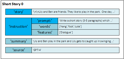
Within a single Json file you will find the 100,000 short stories each stored with the same format containing the following entries as described by [3]:

Story: the story portion contains the actual short story text created using the source model, instructions, and summary.

Instruction: the instruction contains a prompt used to prepare the model, a list of words to be included in the story, and features describing the story’s attributes.

Summary: a summary of the story used to create the actual full story text along with the instructions.

Source: the source is the source model used to create and summarize the short story.

When training the Instruct Llams2 model, both the story and instruction:prompt portions of the data are used.

Pre-Tokenizing The Data

Pre-tokenizing is the process of selecting and converting the raw text into tokens where a token is a numeric index value that references a specific sub-text value within the vocabulary. For example, a 26-character based vocabulary would have twenty-six entries and therefore token values from 0 to 25. As you can imagine, large language model vocabularies are much larger for they consist of not only the characters used but also numerous combinations of the characters used. A common tokenization algorithm used to build a vocabulary is called byte-pair encoding [4] [5].  This type of tokenization method is used by the Llama models, including the Instruct Llama2 model which builds a vocabulary of 32,000 entries, like Baby Llama.

During tokenization of the Instruct Llama model, the following steps occur.

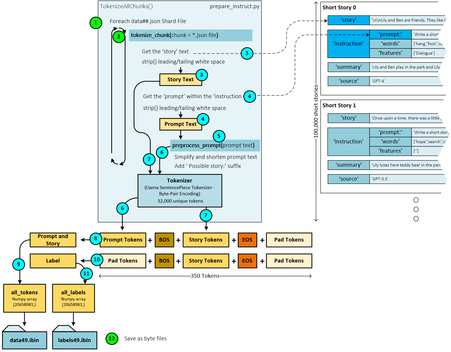
1. For each Json file (e.g., json), …
2. … the tokenize_chunk() function tokenizes each of the 100,000 short stories within the Json file.
3. During tokenization, first the story text is extracted from the shard and stripped of leading/trailing white space.
4. Next, the instruction prompt is extracted from the shard and stripped of leading/trailing white space.
5. The prompt is then pre-processed with the preprocess_prompt() function which simplifies and shortens the instruction.
6. The shortened instruction prompt is then tokenized with the Tokenizer using the byte-pair tokenization process implemented by the SentencePieceProcessor which is part of SentencePiece.
7. Then the story text is tokenized using the same byte-pair tokenization process implemented by the SentencePieceProcessor.
8. The input tokens (called Prompt and Story) are constructed by combining the prompt tokens + a BOS token + the story tokens + an EOS token + any Pad tokens necessary to fill out the full 350 token sequence length.
9. The target tokens (called Label) are constructed by combining a set of Pad tokens for the number of prompt tokens + a BOS token + the story tokens + an EOS token + any Pad tokens necessary to fill out the full 350 token sequence length. Note, the initial Pad tokens are used to tell the model to ignore the input prompt tokens so that the model does not increase the loss based on bad prompts.
10. The Prompt and Story tokens created from each shard are then added to the all_tokens
11. And the Label tokens created from each shard are added to the all_labels
12. Upon completing the tokenization of all shards, the all_tokens and all_labels lists are saved as a byte files to the corresponding data and label files, respectively. For example, the tokenized json shards are saved to the data49.ibin binary data file containing the Prompt and Story tokens and the label49.ibin binary label file containing the Label tokens.

Training From Scratch

When training the Instruct Llama model from scratch, the process is very similar to training the Baby Llama model with several differences highlighted in light green. Initially, like the Baby Llama, the model contains randomly initialized weights that have no learned knowledge. Like the Baby Llama model, the Instruct Llama model is trained to predict the next token given the set of training input tokens. Unlike the Baby Llama model, the inputs to the Instruct Llama model contain an instruction prompt followed by the story text.

During training, the pre-tokenized tokens are used to train the model with the following steps occurring. Steps that differ from the original Baby Llama training process are preceded with a ‘**’ string.

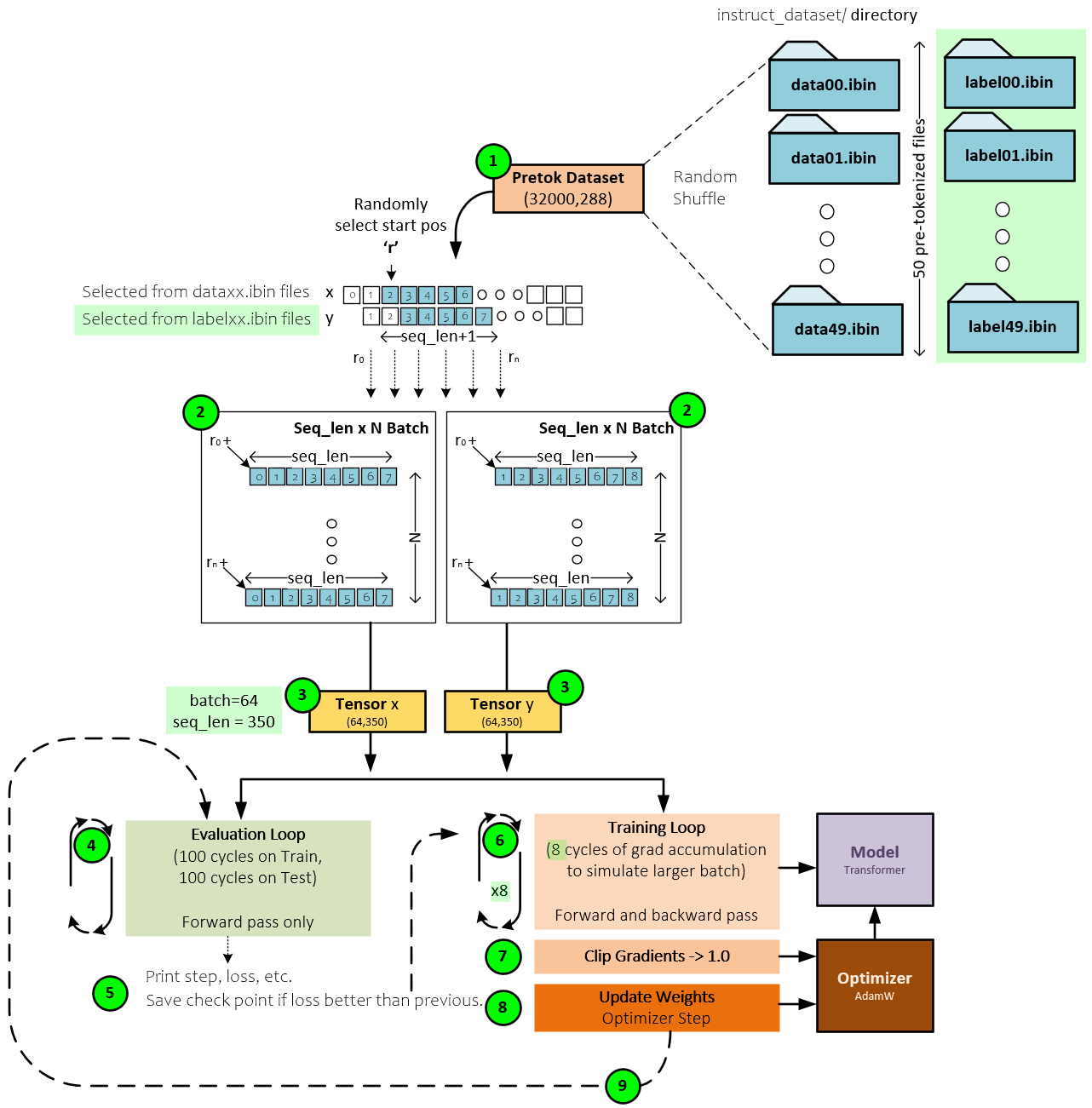
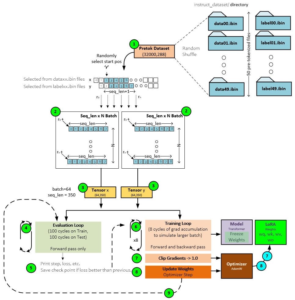
1. **The Pretoke Dataset loads each pre-tokenized data*.ibin data file and label*.ibin label file into two memory mapped files that are used when needed and randomly selects the starting point ‘r’ from within the synchronized file data. A seq_len of tokens is loaded from the ‘r’ starting point and stored as the current line in the batch being built. Each line of data and label are seq_len in length. The X tensors are loaded from the data file and the Y tensors are loaded from the label file. To predict the next token, the Y tensors are offset one token forward in the sequence from that of the X input sequence.
2. A grid of token sequences, each of seq_len in length, are stacked to create the X batch, and Y batch where each sequence in the Y batch is shifted by one token forward in corresponding X sequence of tokens.
3. **The X and Y batches of tokens are placed into Tensors of size (64,350) corresponding to a batch size of 64 and sequence length of 350.
4. The X and Y batches are then sent through the evaluation loop that calculates the current training (using the X batch) and testing (using the Y batch) losses. This loop runs for one hundred iterations and the losses calculated are averaged.
5. The losses are printed for output and if the test loss is better than the previous loss, the current model check-point weights are saved to disk.
6. **Next, the training loop is entered to train the model. To simulate a larger batch size, the training loop runs eight cycles and accumulates the gradients at each step. These gradients will later be used to alter the model weights which is how the model leans. The Instruct Llama model runs eight cycles instead of the four running in the Baby Llama model because of the smaller batch size used by the Instruct Llama model which is ½ the size of the 128-batch size used in the Baby Llama model.
7. Next, the gradients are clipped to values no larger than 1.0 for model stability.
8. And, then the optimizer is used to update the model weights using the learning rate, momentum, weight decay and the optimizer algorithm used. Baby Llama uses the AdamW [6]
9. After updating the weights, the training loop continues and at certain iterations re-enters the evaluation loop, or otherwise continues to the next training loop.

Training continues until a sufficiently low and acceptable loss value is observed in the testing dataset that does not diverge from the training loss – which usually indicates overtraining.

Upon completion of the training, the trained weights are ready to use for story generation.

Fine-Tune Training with LoRA

When using large language models, training the entire model, or even fine-tuning by training a portion of the model is often prohibitively expensive. Low-Rank Adaption (LoRA) [10] offers a more efficient way to fine-tune a large language model by only training a small sub-set of new weights that augment key weight tensors within the model.

LoRA changes the way specific, strategically selected Linear layers operate. All layer weights are frozen when using LoRA which speeds up training and dramatically shrinks the required number of learnable parameters. In fact, Hu et. al. states, “LoRA can reduce the number of trainable parameters by 10,000 times and the GPU memory requirement by 3 times.” [10]

How Does LoRA Work?

Out of the several ways to implement LoRA [11] [12] [13], the Instruct Llama Model uses the method proposed by Chang [12] who employs the PyTorch parameterization feature to call the LoRALinear layer each time the associated weight is accessed, such as during the forward pass.

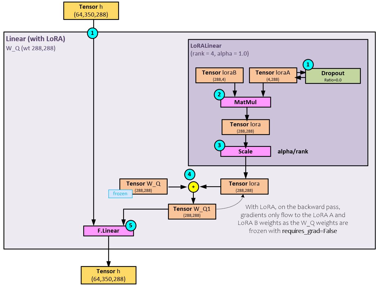
During the forward pass within a Linear Layer using LoRA, the following steps occur.

1. The input tensor is passed into the Linear Layer, but before using it, the LoRALinear layer starts processing its internal LoRA A and LoRA B weights. The first step taken by the LoRALinear layer is to optionally run the loraA weights through a Dropout layer.
2. Next, a MatMul is performed between the loraB weights of shape (288,4) and loraA weights of shape (4,288) to produce the lora result of shape (288,288).
3. The lora result is then scaled by the alpha/rank parameters to produce the scaled lora tensor.
4. The scaled lora weights are added to the actual Linear layer weights, such as the W_Q weights to produce the W_Q1 LoRA altered weights.
5. When calling the Linear operation of the Linear layer, the new LoRA altered W_Q1 weights are used instead of the original W_Q weights.

When using LoRA, all non-LoRA weights are frozen by setting requires_grad=False for each, which directs the backward pass to only store the gradients calculated for the loraA and loraB weights. This is where the 10,000 x savings in trainable parameters originates from. Gradients are still calculated and propagate back through the network, but only the loraA and loraB gradients are stored and used to update their weights via the optimizer.

To learn more about other implementations of LoRA, including the original implementation proposed by Hu et. al., see our post on LoRA.

Training/Fine-Tuning with LoRA

When training the Instruct Llama model with LoRA, the process is remarkably like training the Instruct Llama model without, and below the differences are highlighted in light green. Note, during the fine-tuning process, the original weights are not changed – only the LoRA weights are updated during each training cycle.

During training, the pre-tokenized tokens are used to train the model with the following steps occurring. Steps that differ from the original Instruct Llama training process are preceded with a ‘**’ string.

1. The Pretoke Dataset loads each pre-tokenized data*.ibin data file and label*.ibin label file into two memory mapped files that are used when needed and randomly selects the starting point ‘r’ from within the synchronized file data. A seq_len of tokens is loaded from the ‘r’ starting point and stored as the current line in the batch being built. Each line of data and label are seq_len in length. The X tensors are loaded from the data file and the Y tensors are loaded from the label file. To predict the next token, the Y tensors are offset one token forward in the sequence from that of the X input sequence.
2. A grid of token sequences, each of seq_len in length, are stacked to create the X batch, and Y batch where each sequence in the Y batch is shifted by one token forward in corresponding X sequence of tokens.
3. The X and Y batches of tokens are placed into Tensors of size (64,350) corresponding to a batch size of 64 and sequence length of 350.
4. The X and Y batches are then sent through the evaluation loop that calculates the current training (using the X batch) and testing (using the Y batch) losses. This loop runs for one hundred iterations and the losses calculated are averaged.
5. The losses are printed for output and if the test loss is better than the previous loss, the current model check-point weights are saved to disk.
6. Next, the training loop is entered to train the model. To simulate a larger batch size, the training loop runs eight cycles and accumulates the gradients at each step. These gradients will later be used to alter the model weights which is how the model leans. The Instruct Llama model runs eight cycles instead of the four running in the Baby Llama model because of the smaller batch size used by the Instruct Llama model which is ½ the size of the 128-batch size used in the Baby Llama model.
7. **Next, the LoRA only gradients are clipped to values no larger than 1.0 for model stability. All other weights are frozen and therefore have no stored gradients to clip. The Instruct Llama model applies LoRA to all w_q, w_k, w_v, and w_o. As noted by Hu et. al. in [10], LoRA is also effective when only altering the wq and wv weights for further parameter space savings.
8. **The optimizer is used to update the model LoRA weights only using the learning rate, momentum, weight decay and the optimizer algorithm used. Baby Llama uses the AdamW [6] All non-LoRA weights are frozen and therefore are not updated.
9. After updating the weights, the training loop continues and at certain iterations re-enters the evaluation loop, or otherwise continues to the next training loop.

Training continues until a sufficiently low and acceptable loss value is observed in the testing dataset that does not diverge from the training loss – which usually indicates overtraining.

Upon completion of the training, the trained weights are ready to use for story generation.

Instruct Story Generation

Once trained, the Instruct Llama model can be instructed to generate short stories. For example, the user might send the model the following:

“Write a story. In the story, try to use the verb ‘run,’ the noun ‘flower’ and the adjective ‘clever.’ Possible story:”

From the input, the model generates a story that meets the instruction. This is different from the Baby Llama mode which just generates a story but does not consider any instructions.

When generating a story based on a given instruction, the following steps occur in the Instruct Llama model.

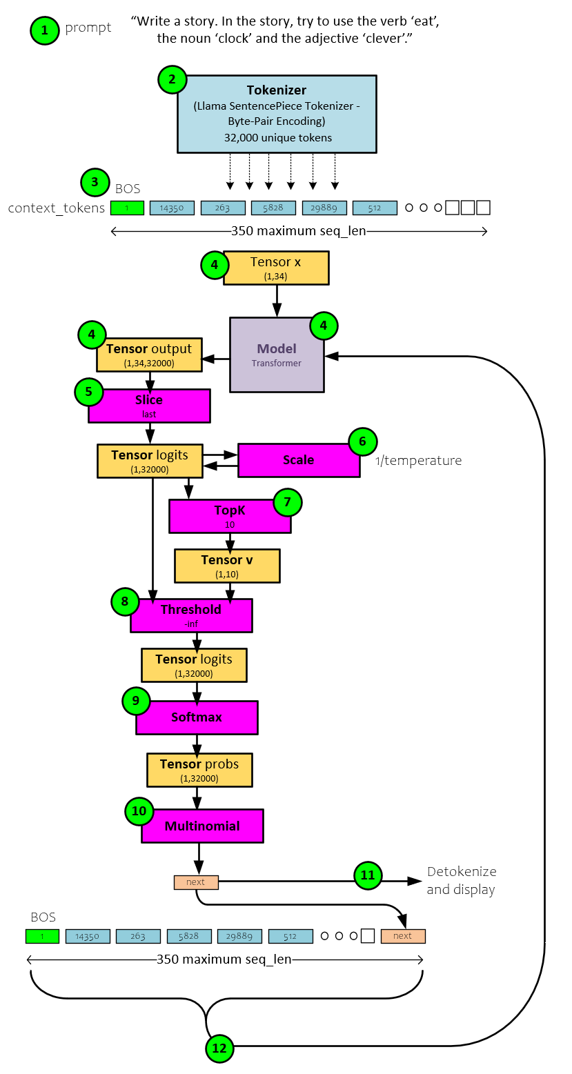
1. The user enters the prompt with an instruction like “Write a story. In the story, try to use the verb ‘eat,’ the noun ‘clock’ and the adjective ‘clever.’
2. The Tokenizer uses the byte-pair encoding algorithm to tokenize the inputs.
3. And the BOS (begin of sentence) token is pre-pended to the tokens to create the input context_tokens.
4. The full set of context_tokens are placed in the X tensor of shape (1,34) and run through the model which produces the output tensor of logits with size (1,34,32000).
5. The last logit is sliced from the output tensor to become the logits tensor for the predicted next token.
6. The logits tensor is scaled by 1/temperature…
7. … and the topK = 10 values are selected, ordered, and placed in the v
8. All values within the logit’s tensor less than the smallest topK value are set to -inf.
9. The logits tensor with clipped values is sent to the Softmax which only focuses on the 10 most important values.
10. A Mutlinomial is run to select the next predicted value based on the probabilities created by the Softmax to produce the next predicted token.
11. The next token is detokenized for display and then the token itself is appended to the input tokens. If the input tokens + the new tokens exceed the sequence length, the first token is removed.
12. The input tokens + newly predicted token is then sent back to the model for processing and the cycle continues until the EOS token is received.

Instruct Llama Model (without LoRA)

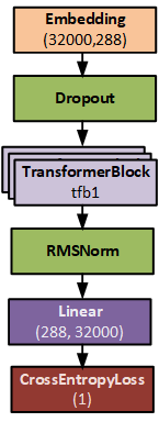
The Instruct Llama model is the same as Baby Llama model except for the batch size and sequence length used. The Instruct Llama model uses batch_size=64 and seq_len=350 whereas the Baby Llama model uses batch_size=128, seq_len=256. Other than those settings, like Baby Llama, this model is a scaled down version of the same model architecture used by the full Llama2 7B and Llama2 13B models. The main difference between the models is that the number of layers and model dimensions are much smaller in the Instruct and Baby Llama models.

When processing the Instruct Llama Model, the following steps occur – note the differences between this model and Baby Llama are just in the batch and sequence sizes.

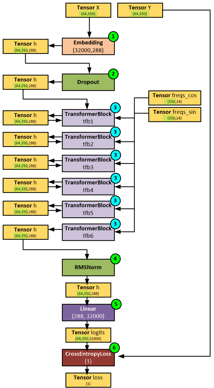
1. **First, the input batch of tokens in the X tensor of input tokens is sent to the Embedding layer which converts each token into a 288-dimensional embedding. Embeddings are used to spatially separate each of the 32000 potential token values. The output of the embedding process is placed in the h tensor of shape (64, 350, 288) which corresponds to a batch size of 64 sequence length of 350 tokens, each with a dimension of 288 for the embedding. Larger Llama2 models use an embedding size of 4096.
2. Next, the h tensor is passed through a Dropout layer to help regularize the model.
3. And then the h tensor is run through the stack of TransformerBlock layers that make up the foundation of the overall model. As you will see later, each TransformerBlock contains the attention mechanism as discussed by Vaswani et. al. [7], which is where the main knowledge learning of the model occurs. The main difference between the Baby Llama Model and larger models such as the 7B Llama2 model is that Baby Llama uses 6 TransformerBlocks corresponding to the 6 layers, whereas the 7B Llama2 Model uses 32 TransformerBlocks corresponding to its 32 layers. Also, note at this stage, the freqs_cos and freqs_sin tensors are fed into each TransformerBlock – these two tensors are used to add positional encoding to the Q and V tensors during CausalSelfAttention (discussed later).
4. After the last TransformerBlock the h tensor is normalized with the RMSNorm [8] layer for model stability.
5. **Then the h tensor is processed by a straight Linear layer which converts the h tensor into the logits of shape (64,350,32000) where each of the 32000 values each represent a probability associated with the predicted token to be next within the vocabulary set.
6. A CrossEntropyLoss [9] layer is used to calculate the loss which then feed into the backward pass to calculate the gradients that later update the weights to facilitate model learning.

Like the Baby Llama model, the TransformerBlock layer is one of the key layers in the model as it makes up the main area of learning in the Transformer model. Given that the same model is used as Baby Llama, we encourage you to visit our previous post to learn more about the details of the TransoformerBlock works.

Instruct Llama Model with LoRA

The Instruct Llama model with LoRA is the same as Instruct Llama model except for the addition of the LoRA enabled weights. Instruct Llama adds LoRA to each w_q, w_k, w_v, and w_o weight within each of the TransformerBlock layers.

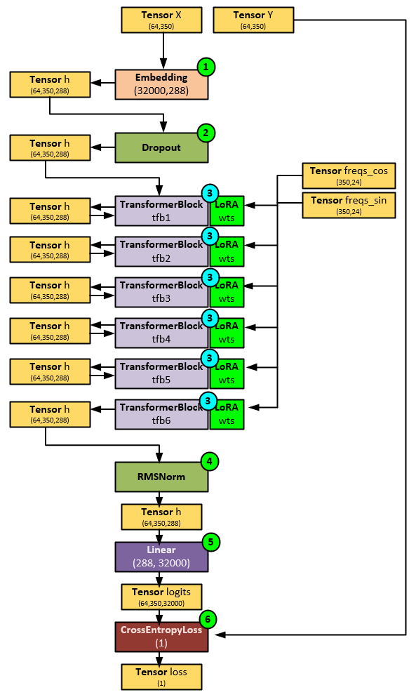
When processing the Instruct Llama Model, the following steps occur – note the differences between this model and Baby Llama are just in the batch and sequence sizes.

1. First, the input batch of tokens in the X tensor of input tokens is sent to the Embedding layer which converts each token into a 288-dimensional embedding. Embeddings are used to spatially separate each of the 32000 potential token values. The output of the embedding process is placed in the h tensor of shape (64, 350, 288) which corresponds to a batch size of 64 sequence length of 350 tokens, each with a dimension of 288 for the embedding. Larger Llama2 models use an embedding size of 4096.
2. Next, the h tensor is passed through a Dropout layer to help regularize the model.
3. **And then the h tensor is run through the stack of TransformerBlock layers that make up the foundation of the overall model. As you will see later, each TransformerBlock contains the attention mechanism as discussed by Vaswani et. al. [7], which is where the main knowledge learning of the model occurs. The main difference between the Instruct Llama model with and without LoRA is that the LoRA enabled version has additional LoRA weights added to each of the w_q, w_k, w_v and w_o Linear layers within the CausalSelfAttention layers (discussed later) used within each TransformerBlock
4. After the last TransformerBlock the h tensor is normalized with the RMSNorm [8] layer for model stability.
5. Then the h tensor is processed by a straight Linear layer which converts the h tensor into the logits of shape (64,350,32000) where each of the 32000 values each represent a probability associated with the predicted token to be next within the vocabulary set.
6. A CrossEntropyLoss [9] layer is used to calculate the loss which then feed into the backward pass to calculate the gradients that later update the weights to facilitate model learning.

When using LoRA, the TransformerBlock layer is one of the key layers in the model as it makes up the main area of learning in the Transformer model.

TransformerBlock Layer (with LoRA)

Whether using LoRA or not, the TransformerBlock layer operates the same and processes each h tensor by applying normalization, attention, and the final feed forward processing. This layer is the backbone of every transformer-based model.

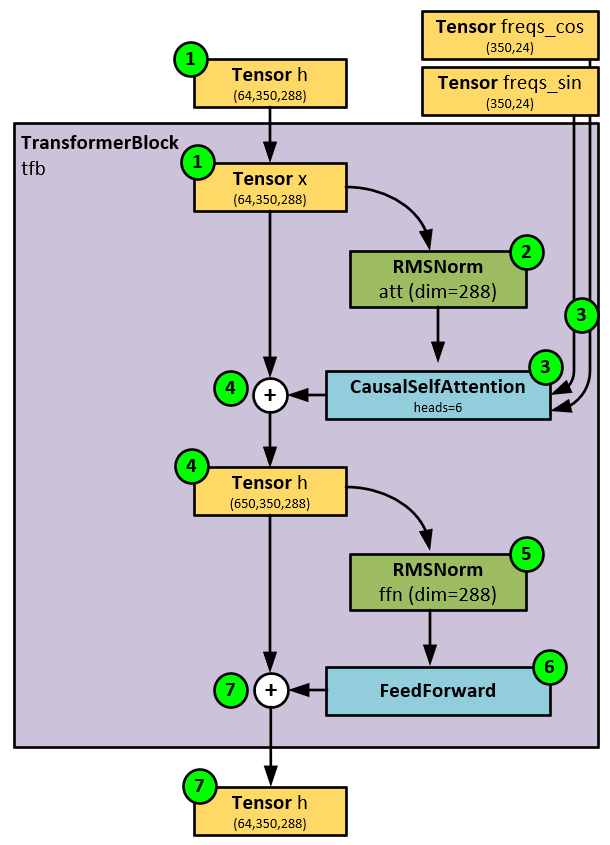
When processing tensors, the TransformerBlock layer takes the following steps.

1. First the h tensor of size (64,350,288) is passed to the transformer block which treats this input tensor as the x
2. Next, the x tensor is normalized using the RMSNorm layer with a dimension of 288, meaning that the last axis of each tensor is normalized. According to [8] a Root Mean Square Layer Normalization (RMSNorm) is computationally more efficient than Layer Normalization in that it “regularizes the summed inputs to a neuron in one layer according to the root mean square (RMS), giving the model re-scaling invariance property and implicit learning rate adaption ability.”
3. In the next step, the CausalSelfAttention applies the time positional embedding using RoPE [14] and then applies self-attention as described by Vaswani et. al. [7]
4. The results from the CausalSelfAttention are then added to the h tensor as a residual.
5. RMSNorm normalizes the h tensor for model stabilization…
6. … and passes the results to the FeedForward final processing.
7. The FeedForward result is added to the h tensor as a residual and returned as an output to the TransformerBlock.

CausalSelfAttention Layer (with LoRA)

When using LoRA, the main changes occur within the CausalSelfAttention layer that applies attention to the input h tensor and during the process adds the positional information using the freqs_cos and freqs_sin tensors. Differences from the Llama modes without LoRA are preceded with a ‘*’ character.

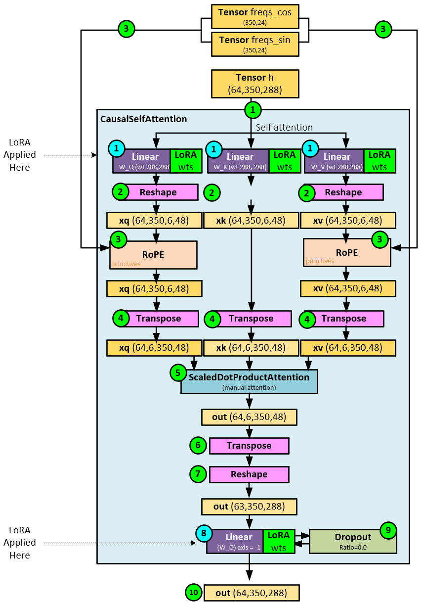
When processing the causal self-attention, the following steps occur.

1. **First the input h tensor is sent to three separate and distinct Linear layers (w_q, w_k, and w_v) to produce the xq, xk, and xv Each Linear layer employs the LoRA update described above where the loraA and loraB weights are used to alter the original W weights.
2. The three xq, xk, and xv tensors are reshaped to allow for processing each of the 6 heads. After reshaping, each of these tensors has a shape of (64,350,6,48) where each of the 6 heads has a dimension of 48.
3. The RoPE algorithm [14] is run on the xq and xv tensors which adds positional information that is essential for the attention processing.
4. The xq, xk, and xv tensors are transposed so that attention can be run along each head. After the transposition, these tensors have a shape (64,6,350,48).
5. Next, the ScaledDotProductAttention is run with the xq, xk, and xv tensors as input and outputs the out tensor of shape (64,6,350,48).
6. The out tensor is then transposed…
7. … and reshaped back to the shape (64,350,288)
8. **The reshaped out tensor is then run through a LoRA enabled Linear layer which uses its internal loraA and loraB weights to alter the W weights…
9. … and optionally a Dropout layer for model stabilization.
10. The final output tensor of the CausalSelfAttention, out has a shape of (64,350,288).

Summary

In summary, the main difference between the Baby and Instruct Llama models resides in the pre-processing stage where the latter pre-processing includes the instruction prompt in the overall tokens saved to each binary token file.

In this post, we have shown how the Instruct Llama model pre-processes its training data by pre-tokenizing the data and instruction prompt, pointing out how this differs from the Baby Llama pre-tokenization process. Next, we described the overall training process used to train the model from scratch, described the model itself, then described how the user instructs the model to create short stories. These designs were derived from both Karpathy’s original Python code in the training.py and model.py files [2] and Sridykhan’s modified Python code found in the instruct_training_from_scratch.ipynb [15].

In addition, we have shown how to fine tune the Instruct Llama model using LoRA which saves parameter space and speeds up learning. The fine-tuning with LoRA designs were derived from Sridykhan’s modified Python code found in the instruct_lora_finetune.ipynb file [15] and Chang’s implementation of minLoRA [12].

To see a description of training Baby Llama which includes much more detail, see our previous training post, and to learn how inferencing takes place using the Llama2.c, see our previous inferencing post. And to learn how the original LoRA implementation by Hu et. al. [10] works, see our previous post on LoRA.

Happy Deep Learning with LLMs!

---

[1] Train from scratch and Fine-tune an Instruct Llama2 model in PyTorch, by Cindy Sridykhan, 2023, Medium

[2] GitHub:karpathy/llama2.c, by Andrej Karpathy, 2023, GitHub

[3] TinyStories: How Small Can Language Models Be and Still Speak Coherent English? by Ronen Eldan and Yuanzhi Li, 2023, arXiv:2305.07759.

[4] Byte-Pair Encoding, Wikipedia

[5] Byte-Pair Encoding: Subword-based tokenization algorithm, by Chetna Khanna, 2021, Medium

[6] Decoupled Weight Decay Regularization, by Ilya Loshchilov and Frank Hutter, 2019, arXiv:1711.05101

[7] Attention Is All You Need, by Ashish Vaswani, Noam Shazeer, Niki Parmar, Jakob Uszkoreit, Llion Jones, Aidan N. Gomez, Lukasz Kaiser, and Illia Polosukhin, 2017, arXiv:1706.03762.

[8] Root Mean Square Layer Normalization, by Biao Zhang and Rico Sennrich, 2019, arXiv:1910.07467

[9] Understanding Categorical Cross-Entropy Loss, Binary Cross-Entropy Loss, Softmax Loss, Logistic Loss, Focal Loss and all those confusing names, by Raúl Gómez, 2018, Raúl Gómez blog.

[10] LoRA: Low-Rank Adaptation of Large Language Models, by Edward J. Hu, Yelong Shen, Phillip Wallis, Zeyuan Allen-Zhu, Yuanzhi Li, Shean Wang, Lu Wang, and Weizhu Chen, 2023, arXiv:2106.09685

[11] GitHub:microsoft/LoRA, by Microsoft Corporation, 2023, GitHub

[12] GitHub:cccntu/minLoRA, by Jonathan Chang, 2023, GitHub

[13] Code LoRA From Scratch, by Lightning.AI, 2023, GitHub

[14] RoFormer: Enhanced Transformer with Rotary Position Embedding, by Jianlin Su, Yu Lu, Shengfeng Pan, Ahmed Murtadha, Bo Wen, and Yunfeng Liu, 2021, arXiv:2104.09864

[15] GitHub:cindysridykhan/instruct_storyteller_tinyllama2, by Cindy Sridykhan, 2023, GitHub