Understanding N-HiTS Time Series Prediction

Non-stationary data is a type of time series data where the statistical properties such as mean, variance, and autocorrelation change over time. In other words, the data exhibits some form of systematic change over time rather than fluctuating around a constant mean or with a constant variance. Non-stationary data can take several forms, including:

1. Trends: The data shows a long-term increase or decrease over time. For example, a time series of annual global temperatures that shows a consistent upward trend due to climate change.
2. Seasonality: The data exhibits regular and predictable patterns that repeat over a specific period, such as daily, monthly, or yearly. For example, retail sales data that spikes during the holiday season every year.
3. Changing Variance: The variability of the data points changes over time. For instance, financial market data might show periods of high volatility followed by periods of low volatility.
4. Structural Changes: The underlying process generating the data changes due to external events, policy changes, or regime shifts. For example, a sudden change in a country’s economic policy might alter the behavior of economic indicators.
5. Random Walk: The data shows a random walk behavior where the value at any time step is a random deviation from the previous time step. Stock prices often exhibit this kind of behavior.

Non-stationarity is important to identify and address because many traditional statistical and machine learning models for time series analysis and forecasting assume stationarity. When the data is non-stationary, these models can produce unreliable or inaccurate predictions. Techniques such as differencing, detrending, or seasonal adjustment are commonly used to transform non-stationary data into a stationary form that is suitable for modeling.

Non-stationary data is challenging to predict with time series models for several reasons:

1. Changing Statistical Properties: Non-stationary data has statistical properties like mean, variance, and autocorrelation that change over time. Traditional time series models, like ARIMA, assume that these properties are constant (stationary) over time, making it difficult to accurately model and predict non-stationary data.
2. Complex Patterns: Non-stationary data often contains trends, seasonality, and other complex patterns that evolve over time. Capturing and forecasting these evolving patterns requires more sophisticated models and techniques.
3. Model Instability: Models trained on non-stationary data can become unstable. Since the underlying process generating the data changes over time, a model that fits well during one period may perform poorly in another period.
4. Overfitting Risk: When dealing with non-stationary data, there is a higher risk of overfitting, as the model might try to capture the noise or temporary patterns instead of the underlying process.
5. Need for Transformation: To manage non-stationarity, data often needs to be transformed to make it stationary. This can involve differencing, detrending, or seasonal adjustment. These transformations add complexity to the modeling process and might not always be straightforward.
6. External Factors: Non-stationary time series data can be influenced by external factors or events (e.g., economic changes, policy shifts, technological advancements) that are not captured by traditional time series models, making accurate prediction more difficult.

To address non-stationarity, more advanced models like those based on machine learning (e.g., LSTM, GRU) or hybrid approaches (e.g., combining ARIMA with machine learning models) are often employed, as they can better capture complex and evolving patterns in the data.

N-HiTS Time-Series Model

The Neural Hierarchical Interpolation for Time Series Forecasting (N-HiTS) model by Challu et al., is designed to improve long-horizon time-series predictions while reducing prediction volatility by using a “novel hierarchical interpolation and multi-rate data sampling techniques.” [1]

By “composing its predictions hierarchically using blocks specialized in different frequencies” the N-HiTS model can “reconstruct non-periodic/stationary signals.” [1]

In this post, we delve into the workings of the N-HiTS model, demonstrating its ability to make time-series predictions with both single target values and with multiple additional covariates. The code used to analyze and explore the N-HiTS models employs the Darts Python library [2] available on GitHub at https://github.com/unit8co/darts.

Dataset Preparation

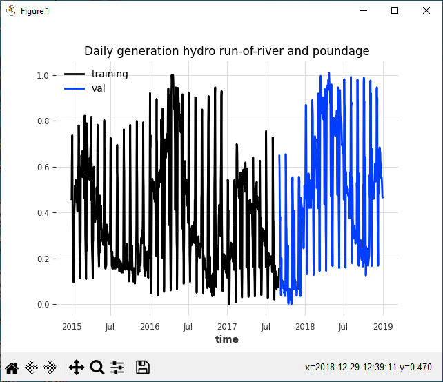
For our studies we use the ‘generation hydro run-of-river and poundage’ column from within the ‘energy_dataset.csv’ found within the Darts ‘datasets’ director. This column of data contains the hourly hydro generations readings from the end of 2014 through 2018.

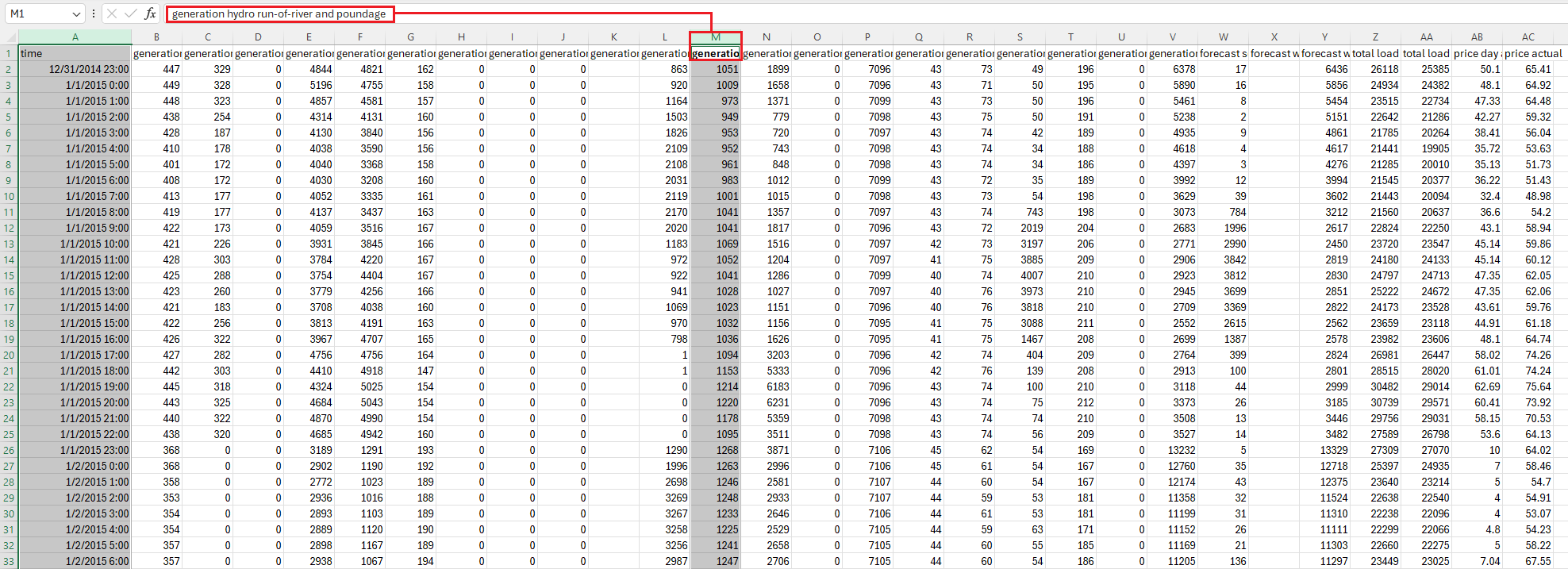
After loading the spreadsheet (1) into a Panda’s dataset (2), a daily average is taken for each day and the daily average data is split (3) into the training and validation data sets of 976 and 486 days of data, respectively.

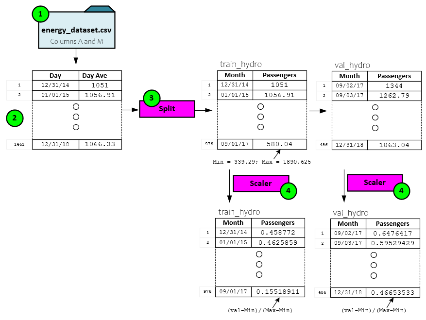
The training and validation datasets are then scaled (4) based on the training set minimum and maximum values to produce the final training and validation scaled datasets each containing values within the range [0.0, 1.0].

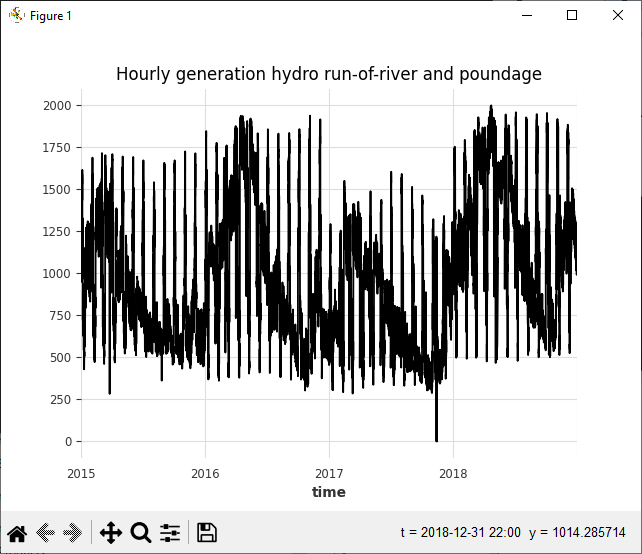
The raw unscaled data shows a semi-periodic data stream as shown in the chart below.

After scaling and splitting the data, the same pattern exists, but now all values are in the range of 0.0 to 1.0 and the first portion of the data comprises the training set with the latter comprising the validation data.

The following code snippet loads, spits, scales and plots the data.

Prediction Results

To predict the hydro production, we trained the N-HiTS model with a previous step size of 30 days and use that period to predict the next 7 days of production. The Darts library [2] constructs a rolling window of data used to build each training batch fed through the model during training. The model was trained for a total of one hundred epochs.

During the training sessions, we trained the model on two different input types. In the first input we only fed the previous 30 days of ‘target’ data to predict the next 7 days. However, in the second training session two time-based covariates (one for the month and the other for the year) were to the targets to see the impact on the training results. Like the targets, both covariates were scaled to the range 0.0 to 1.0.

Time-Based Covariates

The time-based covariates include a monthly and yearly covariate.

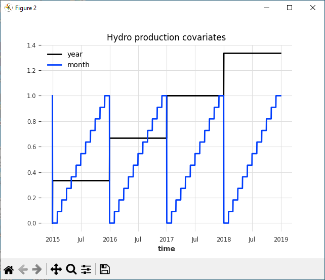
The time-based covariates can be created from the original data series using the following code.

Prediction Results = Without Covariates

Visually the predictions without covariates show a close match to the ground truth values.

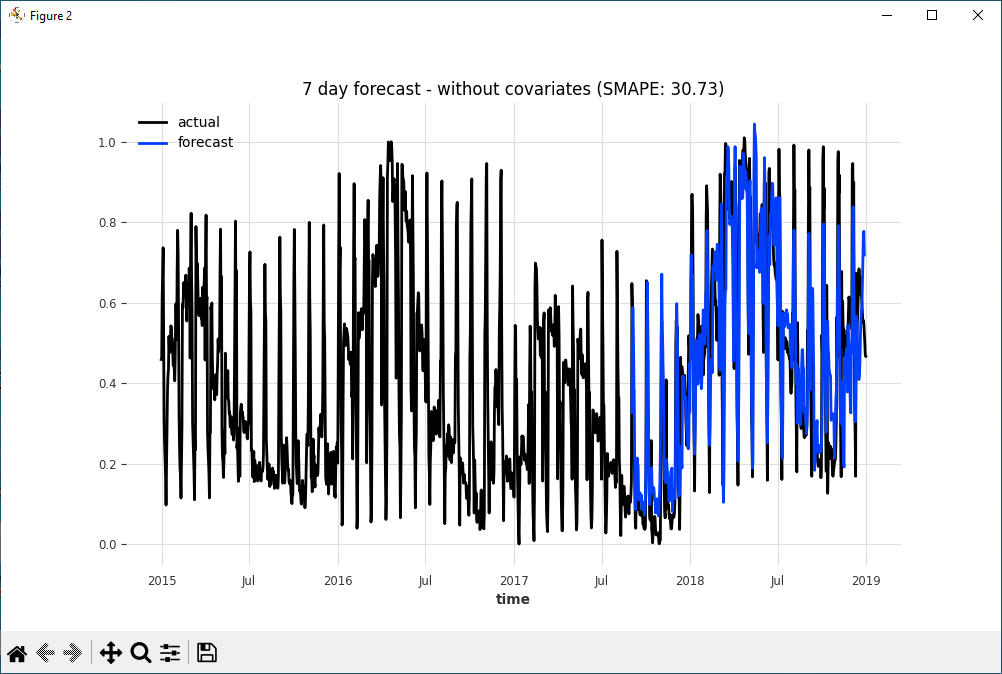
The performance of the model is measured using the SMAPE which equals 30.73.

Prediction Results – With Both Time-Based Covariates

Visually the prediction with the time-based covariates shows less of a match than the predictions without. This does not mean that adding covariates will reduce the overall prediction performance, but instead shows the importance of picking the right covariates.

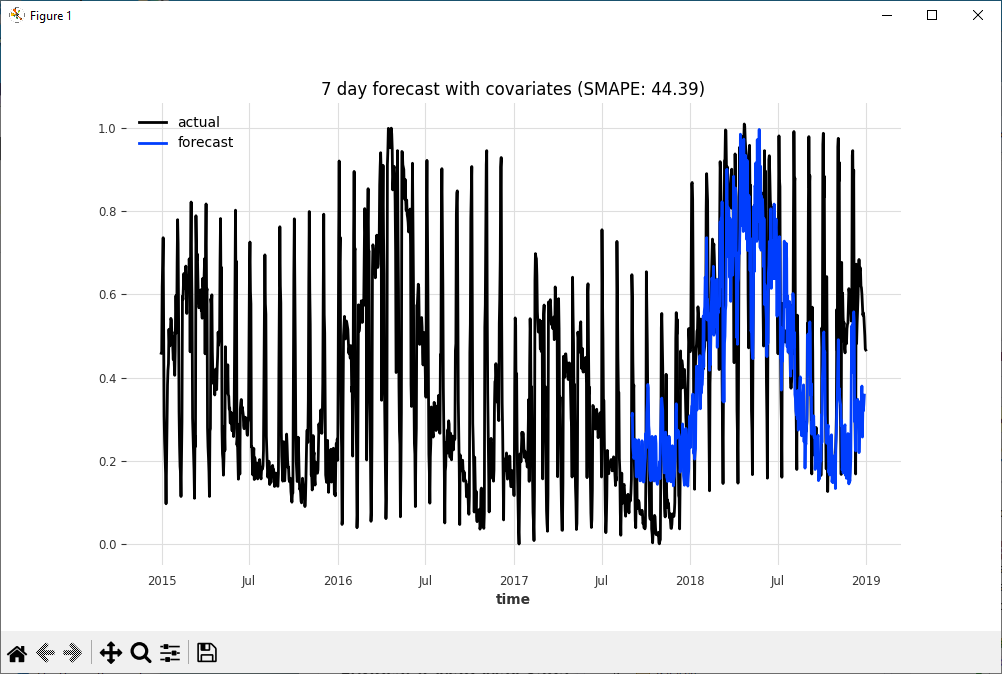
Note the SMAPE of 44.39 observed in the predictions with the two time-based covariates is quite a bit worse than the 30.73 SMAP observed in the predictions without the covariates.

The following code can be used to fit the N-HiTS model using the two additional time-based covariates.

Prediction with Month-Only Time-Based Covariate

Next, we remove the year covariate to see the impact on the predictions with the monthly covariate only.

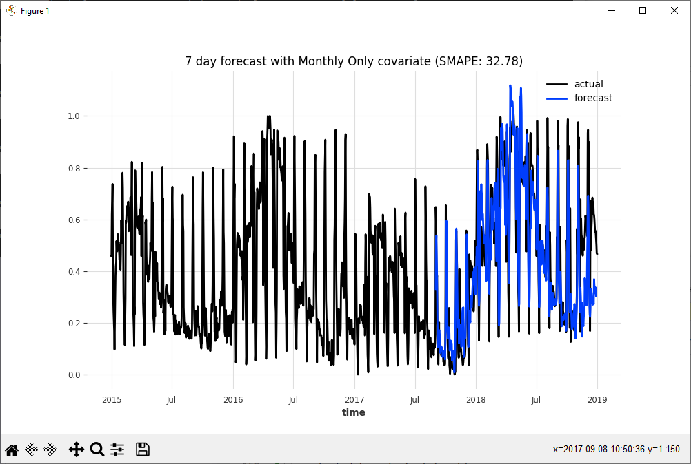
While a significant improvement over the predictions that use both the Year and Monthly time-based covariates with an improved SMAPE of 32.78, the original prediction using no time-based covariates still wins out with a lower SMAPE of 30.73 which demonstrates that the time-based covariates did not help the prediction results in this case.

By comparing the SMAPE and visually inspecting the prediction results we can quickly see which covariates help or hurt the final predictions.

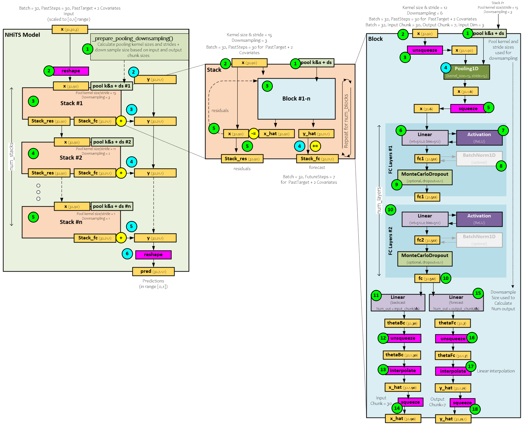
N-HiTS Model

Now that we have seen how the N-HiTS performs when predicting a time-series dataset let us look inside and see how the model works.

The overall model architecture uses a set of ‘Stack’s that each focus on a different frequency within the time-series input data. A focus is placed on each frequency via an internal Pooling layer within a set of one or more ‘Block’s making up each Stack. A ‘Block’ contains one or more groups of Pooling and MLP inner layers that all focus on a specific frequency teased out of the data via the multi-rate signal sampling provided by the Pooling layers’ kernel and stride sizes. Forecast and Backcast Linear layers produce the end results that are then interpolated back into the input shape thus allowing the outputs to be accumulated into the final model prediction.

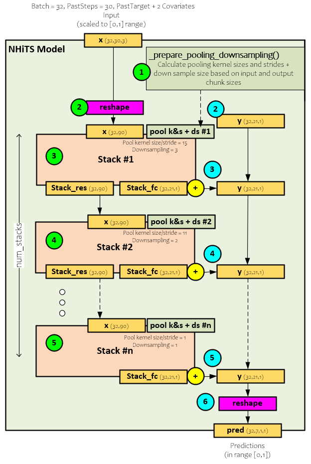
Each time-series data segment loaded by the Darts library is placed into the batch, which is set to 32 time-series segments in the image above, each with 30 past time steps where each past time step contains the target plus two covariates. Above, we show the x (32,30,3) with the target and two covariates for a tail shape of 3. During the forward pass through the N-HiTS model, the following steps occur.

1. Before processing any data, the ideal pooling kernel and stride sizes are calculated along with the down-sampling size for each Stack within the model. For example, the model shown above uses pooling kernel and stride sizes of 15 and 11 in the first two Stacks respectively along with down-sampling sizes of 3 and 2. We will see later how these are used within each Block.
2. The x (32, 30, 3) batch of 30 past time-steps is reshaped by flattening the time-steps and tail data values forming x into the new shape (32, 90). Also, at this time a y (32,21,1) tensor is created and filled with zeros. The y tensor will accumulate the predictions of each Stack which will become the final prediction after the last Stack is processed.
3. The reshaped x (32, 90) is fed into the first Stack which produces the stack_res (32,90) residual values that become the input x (32,90) of the next Stack, and the stack_fc (32,21,1) partial predictions for the frequency processed by the Stack that are added to the y prediction accumulator.
4. The next Stack processes the new x (which are the residuals from the previous Stack) using a different, smaller kernel size and stride along with a smaller down-sampling size. As with the previous Stack, the partial predictions are added to the y prediction accumulator.
5. This process continues through the last Stack which then adds its partial predictions to the y prediction accumulator.
6. The final y prediction accumulation is then reshaped where all covariate predictions are dropped leaving only the predicted future target values for each time-series segment within the batch.

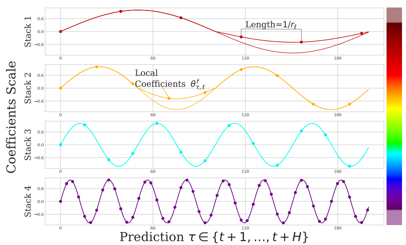
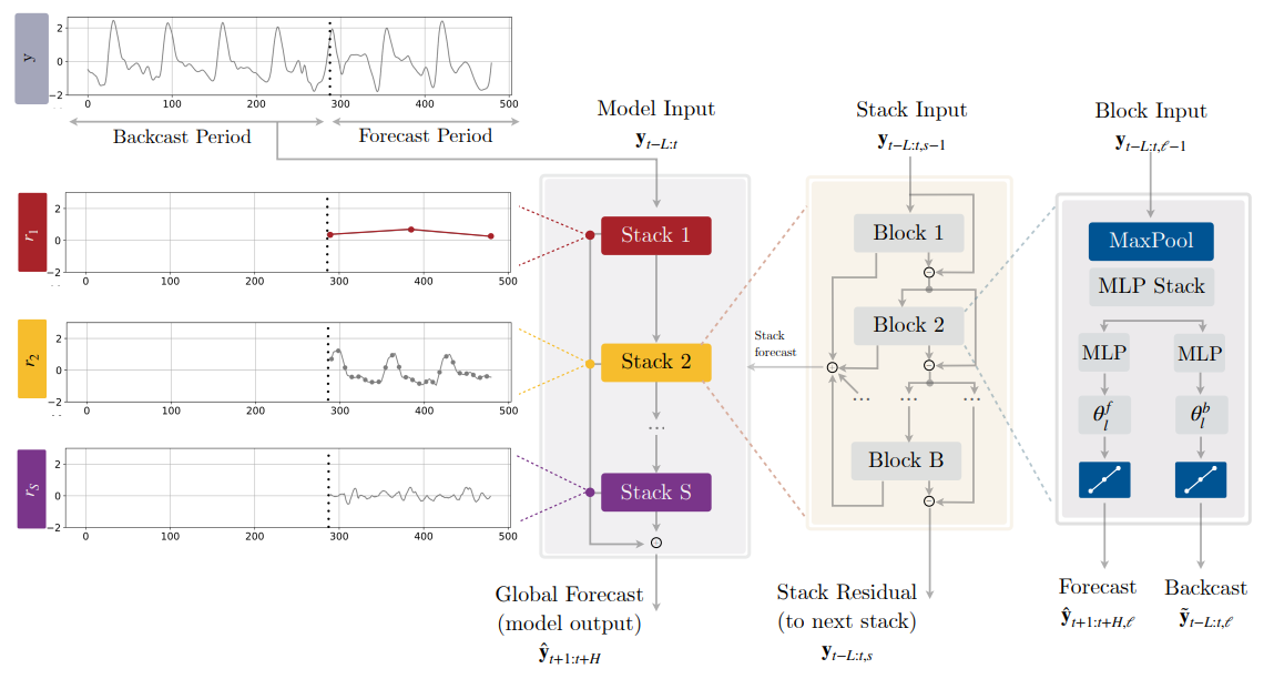
Stack

Each Stack comprises several one or more Blocks. Even though the model studied only uses one Block, each Stack can be configured to use multiple.

When processing each Stack, the following steps occur.

1. During creation, the pool kernel and stride sizes are sent along with the down-sampling size for the Stack to each Block. Note, each Block within the Stack uses the same kernel, stride, and down-sampling sizes.
2. During the forward pass, the x (32,90) input is sent to the first Block for processing.
3. The Block outputs the x_hat (32,90) backcast values and y_hat (32,21,1) forecast predicted values.
4. The y_hat (32,21,1) forecast predicted values are accumulated into the stack_fc (32,21,1) predictions that are output as predictions for the frequency processed by the Stack.
5. The x_hat (32,90) backcast values are subtracted from the x (32,90) input values to produce the residual values that are then fed as input into the next Block. Upon processing the last Block, the x_hat (32,90) residual values become the stack_res (32,90) output residual values.

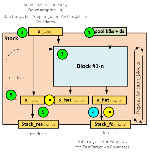
Block

Each Block provides the heart of the prediction for specific frequency in the time-series data. A Pooling layer is used to extract the frequence data that is then processed via a set of FC layer blocks.

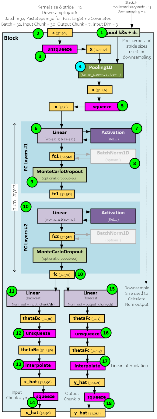
The following steps occur when processing each Block.

1. First, during creation the pooling kernel and stride sizes are used to initialize the Pooling layer and the down-sampling size is used to size the Backcast and Forecast Linear layers.
2. The x (32,90) input values sent to Block contains the 32 time-series segments each with 30 previous time-steps each containing the 3 values (target + 2 covariates).
3. The x (32,90) inputs are un-squeezed to the size (32,1,90) and…
4. … passed to the Pooling layer which (for the first Stack) runs the kernel of size 15 and stride of 15 over the data to produce the new x of size (32, 1, 6), which is…
5. … squeezed back to the size (32,6) and sent to the first FC Layer block #1.
6. Within the first FC Layer block, the Linear layer projects the x (32,6) values to a size of (32,512) by applying its weights and bias.
7. The output of the Linear layer is run through the activation which in this case is a ReLU layer, to produce the fc1 projection output of size (32, 512).
8. The fc1 projection output is optionally run through a BatchNorm1D layer for normalization, …
9. … and then through a Dropout layer, which in this case is a MonteCarloDropout layer with a dropout ratio of 0.10.
10. The final fc1 (32,512) result is then sent to the next FC Layer block and this process continues until the last FC Layer block processes the fc
11. The final fc (32, 512) outputs are non-linearly regressed backward via the backcast Linear layer to produce the thetaBc (32,30) “MLP coefficients that learns [a] hidden vector [that is] used to synthesize the backcast outputs” [1] of the Block.
12. The thetaBc (32,30) is un-squeezed to size (32,1,30) …
13. … and interpolated to produce the x_hat (32,1,90) …
14. … and squeezed to the final x_hat (32, 90) which is an output of the Block.
15. On the forecast side, the final fc (32,512) output is non-linearly regressed forward via the forecast Linear layer to produce the thetaFc (32,7) “MLP coefficient that learns [a] hidden vector [that is] used to synthesize the forecast outputs” [1] of the Block.
16. The thetaFc (32,7) is un-squeezed to size (32,1,7) …
17. … and interpolated to produce the y_hat (32,1,21) …
18. … and squeezed to the final y_hat (32,21) which is an output of the Block for the forward predictions.

Full Model

To view the full model, click on the image below.

Summary

“In most multi-horizon forecasting models, the cardinality of the neural network prediction equals the dimensionality of horizon, H. For example, in N-BEATS |θfl| = H; in Transformer-based models, decoder attention layer cross-correlates H output embeddings with L encoded input embeddings (L tends to grow with growing H). This leads to quick inflation in compute requirements and unnecessary explosion in model expressiveness as horizon H increases.” [1] The hierarchical nature of N-HiTS allows each Stack to focus its Blocks on different frequencies “based on controlled signal projections, through expressive ratios, and interpolation of each Block.” [1] This not only helps learn changing patterns within non-stationary data but does so with reduced compute requirements thus allowing for faster training times.

In this post, we discussed the N-HiTS model for predicting non-stationary time-series data. We demonstrated how this model can predict univariate time-series data and the benefits and drawbacks of adding covariates to the predictions. In addition, we demonstrated how to tell if additional covariates help or hurt the predictions by comparing the prediction outcomes. And finally, we discussed a thorough walk-through of the model, showing how the data flows from one layer to the next to perform the predictions offered by the hierarchical architecture of the model specifically design to detect different frequencies within the data.

Happy deep learning with N-HiTS!

---

[1] N-HiTS: Neural Hierarchical Interpolation for Time Series Forecasting, by Cristian Challu, Kin G. Olivares, Boris N. Oreshkin, Federico Garza, Max Mergenthaler-Canseco, and Artur Dubrawski, 2022, arXiv 2201:12886

[2] Darts: User-Friendly Modern Machine Learning for Time Series, by Julien Herzen, Francesco Lässig, Samuele Giuliano Piazzetta, Thomas Neuer, Léo Tafti, Guillaume Raille, Tomas Van Pottelbergh, Marek Pasieka, Andrzej Skrodzki, Nicolas Huguenin, Maxime Dumonal, Jan Kościsz, Dennis Bader, Frédérick Gusset, Mounir Benheddi, Camila Williamson, Michal Kosinski, Matej Petrik, and Gaël Grosch, 2022, JMLR