

While completing the MyCaffe implementation of the transformer encoder/decoder model for language translation, we ran into a very difficult bug to fix – in fact it was the kind of bug feared most when developing a model for with this bug everything appeared to work as expected when training. Yet, the model would train up to 25-26% accuracy and then hit a wall where the accuracy would not improve any further. Bugs occurring in the learning process are difficult to find for the data of the forward pass and gradients of the backward pass may appear to be correct, and their numbers are usually very small.
In this section we discuss a few techniques to not only isolate but fix the bugs causing our learning to stall.
Verify New Model’s Data Against a Working Model’s Data
Fortunately, our implementation of the transformer encoder/decoder model is based on a pre-existing model written in PyTorch by Jaewoo (Kyle) Song and available under MIT license at GitHub devjwsong/transformer-translator-pytorch. Using the PyTorch auto-grad custom functions, we recrafted this working model to save all weights, input and output data passing through each layer of the model. The weights were loaded into the MyCaffe model (which has a byte compatibility with PyTorch) using the Blob.LoadFromNumpy() function which supports the Numpy file format. Now that the MyCaffe model had the same initialization state as the PyTorch version, we compared each input and output of each layer with those of the Pytorch model using the MyCaffe Blob.Compare() method. Using this technique helped us eliminate several initial bugs in the MyCaffe implementation. In particular, the custom PyTorch auto-grad functions helped us develop and diagnose the direct gradient implementations in MyCaffe. Given that values in both the forward pass and backward pass are very small, we dramatically boosted the loss weight (e.g., x 1000000) to force larger values that could then be compared more easily and eliminate most floating-point precision issues. This worked well in most cases and allowed us to verify exact results in the MyCaffe implementation, yet several layers still had differences which we attributed to floating point precision differences.
Yet, even after comparing every layer, our model was still stuck at the 25% accuracy wall.
Verify Working Model Data Inputs with New Model
Next, we sought to isolate the problem by determining if the issue was in the input data processing (via sentence piece) or within the model itself. Since we had created a custom sentence piece tokenizer, the issue certainly could have been in the data it generated. Using Python.net, we replaced the main PyTorch model with the MyCaffe model but used the Python version’s sentence piece tokenizer for data input.
Yet again, the model was still stuck at the 25% accuracy wall which indicated to us that the issue was within our model and not in our sentence piece tokenizer.
Replace Individual Layers in Working Model
To create the transformer encoder/decoder model several new layers were added to MyCaffe, including a new LogSoftmax, NLLLoss, PositionEncoder, LayerNorm, MultiheadedAttention, and TransformerBlock (for both encoder and also decoder). Most layers were verified with exact results to those produced by the PyTorch model – except for the MyCaffe implementation of the LogSoftmax, Softmax and LayerNorm layers. For these three layers, we swapped the existing model’s layer with the MyCaffe implementation and were able to verify satisfactory results confirming that differences observed in these layers were in fact due to small floating point precision differences.
Yet, even after comparing each of these layers, we were still stuck at the 25% accuracy wall.
Visual Data/Diff Inspection with SignalPop AI Designer
Time for a different approach. As our debugging options on the coding side dwindled, we turned to the visual debugging features of the SignalPop AI Designer.
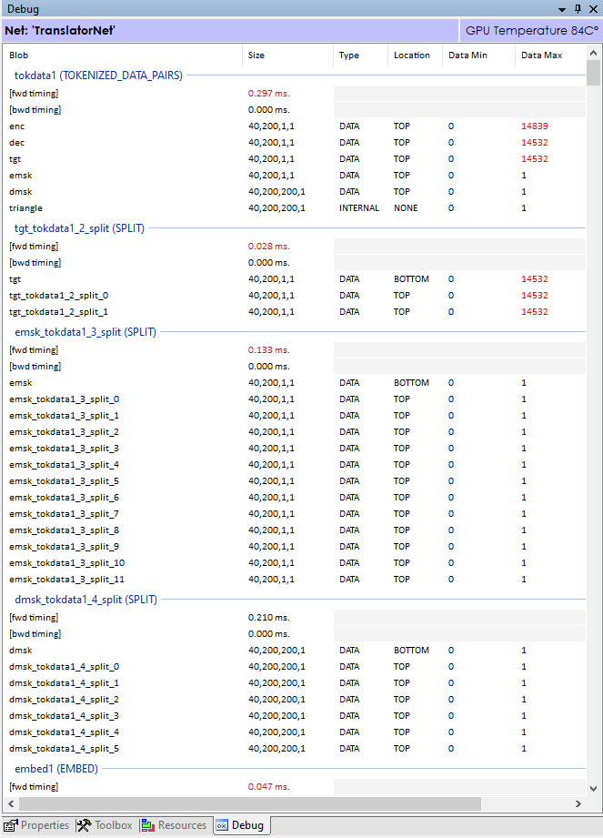
When enabled, the debug window receives data updates for the min/max values of all data flowing through each layer on the forward pass and the diff values (gradients) flowing backward on the backward pass. For example, in the image above, the tokdata1 (TOKENIZED_DATA_PAIRS) layer produces outputs of enc, dec, tgt, emsk, dmsk for the encoder input, decoder input, decoder output (target), encoder mask and decoder mask respectively. As expected, the encoder input, decoder input and decoder output all have values with a range of 0 to less than 16000 as they each contains tokens from the respective source and target vocabularies, each of which having vocabulary sizes of 16000. The encoder and decoder masks fall within the range of [0,1] for the masks are set to 1 in the values we want to focus on and 0 on the values we want to ignore.
Visually inspecting these values can quickly tell whether the values in within an expected number range. For example, if you see the data min/max or diff min/max in the layers at the end of the model increasingly getting larger and larger you know your model is on the path to exploding.
However, when a learning issue is occurring, we must dig deeper and use a more visual approach. One approach offered by the SignalPop AI Designer is to look at the histogram of values in either the data or diff.
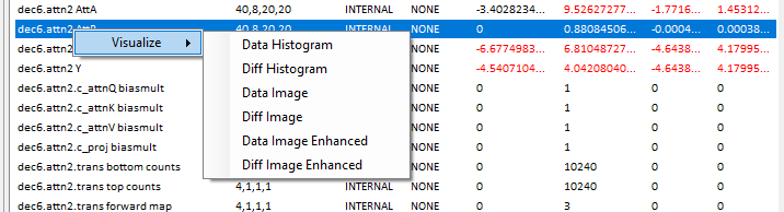
Right clicking on any of the entries in the debug window, such as the dec.attn2 AttB blob (as shown above) allows you to view a histogram on the data or diff values for the blob.
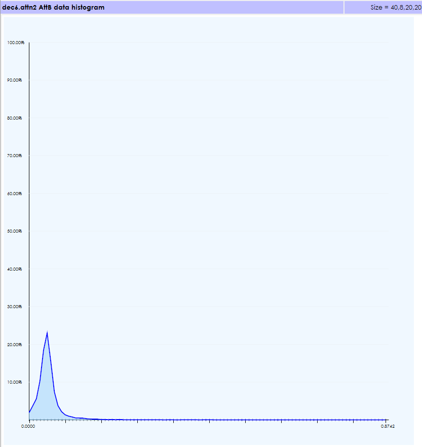
The data histogram shows all values in the range [0,1] which is correct for the AttB blob is the result of running a SoftMax on the AttA blob.
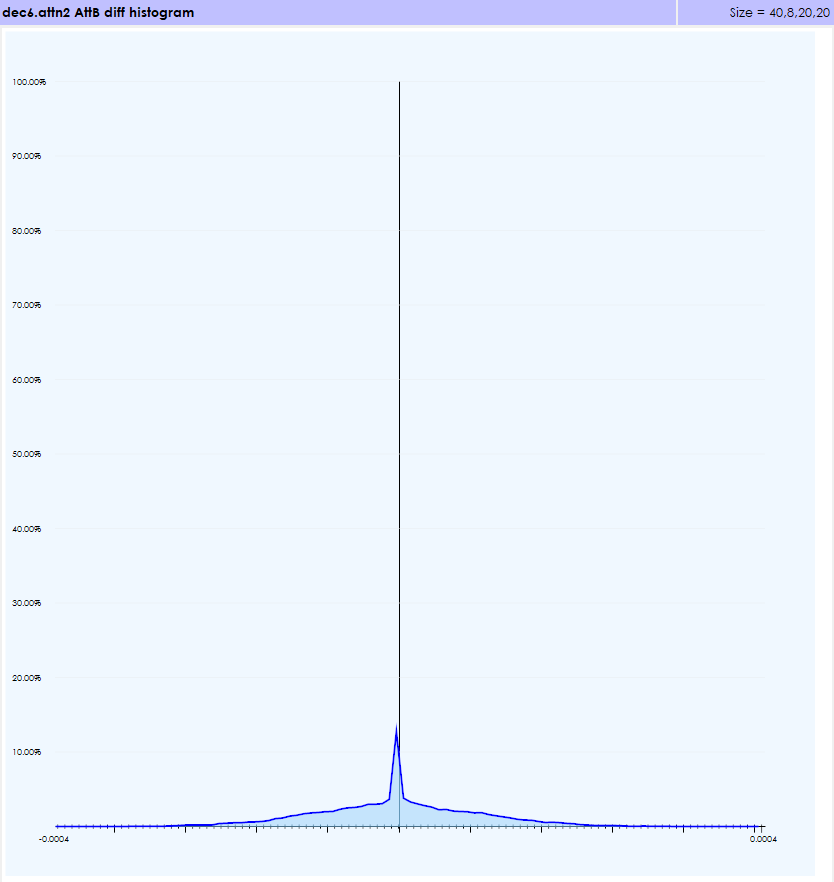
Similarly, the diff values are within an expected range for the Softmax gradients.
Although helpful in determining that values are within the expected ranges we still need to dig deeper for in our case, the numbers within each range were within their expected ranges, but when using the next debug visualization technique our bug became very apparent.
In addition to viewing a histogram of the data and diff data, the data can also be rendered as either a direct image of the data or an enhanced image that colorizes the data based on the data range of the data itself. For this next technique we will use the enhanced images.
When viewing the diff under normal circumstances we would expect to see an image such as the following:
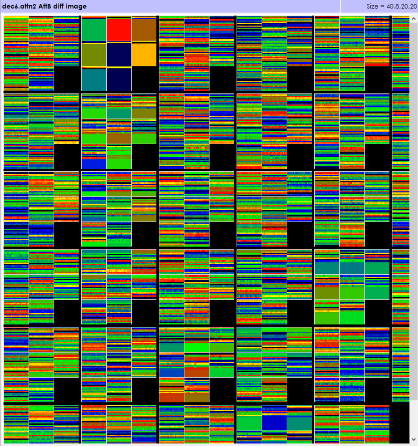
Although these number are very small, we are able to visualize them in the enhanced imaging by coloring each value by their location in the overall data range of the data thus showing us where the data resides. The black boxes are data areas that do not contain any data. As expected, in the image above, each element in the batch is filled with diff values.
However, during our debugging this is the diff image we received.
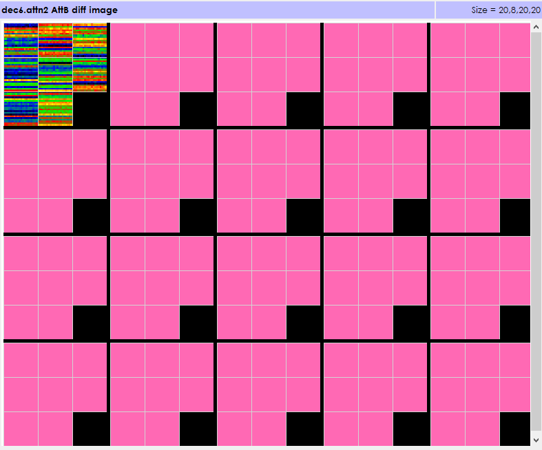
The first element in the batch contains diff values that we would expect. However, the remaining portion of the batch has invalid (pink) values indicating that these diff values are not being produced correctly. By starting from the bottom of the model we were able to isolate where the first bad diff values were produced and fix the bug in that layer thus fixing the learning issue!
The data/diff visualization offered by the SignalPop AI Designer is an invaluable technique to help find difficult learning bugs.
To learn more about the SignalPop AI Designer features, please see the SignalPop AI Designer Getting Started guide available in the SignalPop Developer Document area.