

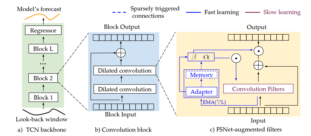
In this blog post, we evaluate from a programmer’s perspective, the FSNet described in “Learning Fast and Slow for Online Time Series Forecasting” by Pham et. al., 2022.[1] The authors of FSNet describe the model as inspired by “Complementary Learning Systems (CLS) theory” to provide “a novel framework to address the challenges of online forecasting” by improving “the slowly learned backbone by dynamically balancing fast adaptation to recent changes and retrieving similar old knowledge.”
Data Processing
Out of the several data sources the paper references, we focus primarily on the ETTh2.csv dataset of electricity usage available from the GitHub:zhouhaoyi/ETDataset open-source project [2].
The ETT dataset contains records comprising a time stamp and 7 additional data fields for the following electricity usage related data.
HUFL – high use full load
HULL – high use low load
MUFL – medium use full load
MULL – medium use low load
LUFL – low use full load
LULL – low use low load
OT – oil temperature.
In this dataset, 2881 records are used for training and 10781 records are used for testing, which includes online training.
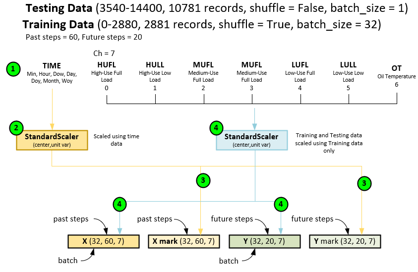
When pre-processing the dataset, the following steps occur.
- First the dataset is loaded with the time + 7 fields per record.
- The time field is scaled using the StandardScaler run both in the training and testing datasets.
- The time scaling produces the X mark and Y mark
- Next, the other 7 data fields are fitted to a StandardScaler with the training data then scaled across both the training and testing data. Note the standard Scaler performs a data centering that is fit to the unit variance. The fit values are placed in the X input and Y target data blobs. These blobs are fed into both the training and testing cycles.
Training Process
The training process uses a standard batch processing forward pass coupled with a loss calculation using the MSE Loss that is then fed through the backward pass to calculate the gradients that are then applied using an AdamW optimizer. A batch size = 32 is used during the initial training process.
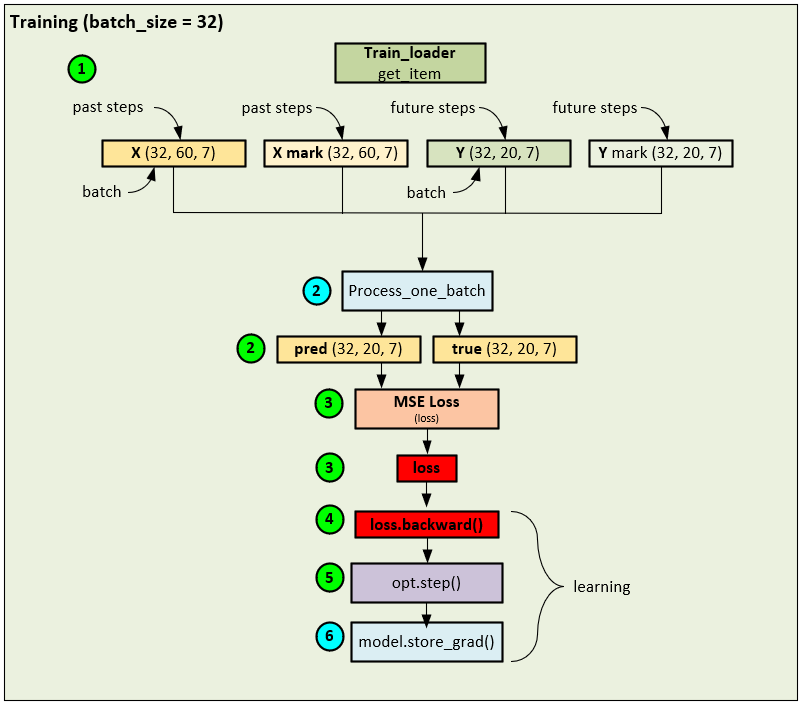
During the training phase, the following steps occur.
- A data loader is used to collect shuffled data records to build each batch of 32 that make up the X, X mark, Y and Y mark Note, 60 past steps are used in the input data and 20 future steps are used in the targets where the X and Y tensors contain the 7 input fields (HUFL, HULL, MUFL, MULL, LUFL, LULL and OT). The X mark and Y mark tensors are filled with seven-time fields related to the current time of the record which include the Minute, Hour, Day of Week, Day, Day of Year, Month and Week of Year.
- The input and target tensors are fed into the Process_one_batch function which takes care of running the model (and in the online training case, preforms a single batch training cycle). The Process_one_batch function produces the pred and true tensors containing the predicted and ground truth values respectively.
- The pred and true tensors are fed into the MSE Loss to produce the loss value.
- And the loss value is used to run the backward pass that propagates the error back through the network to calculate the gradients at each layer.
- An AdamW optimizer is used to calculate and apply the final gradients to the weights of each trainable parameter.
- In a final step, the model’s store_grad function is called to update a special convolutional gradient and determine whether to trigger the fast-learning update mechanism.
This standard batch training is used to ‘warm-up’ the network to the expected patterns in the dataset.
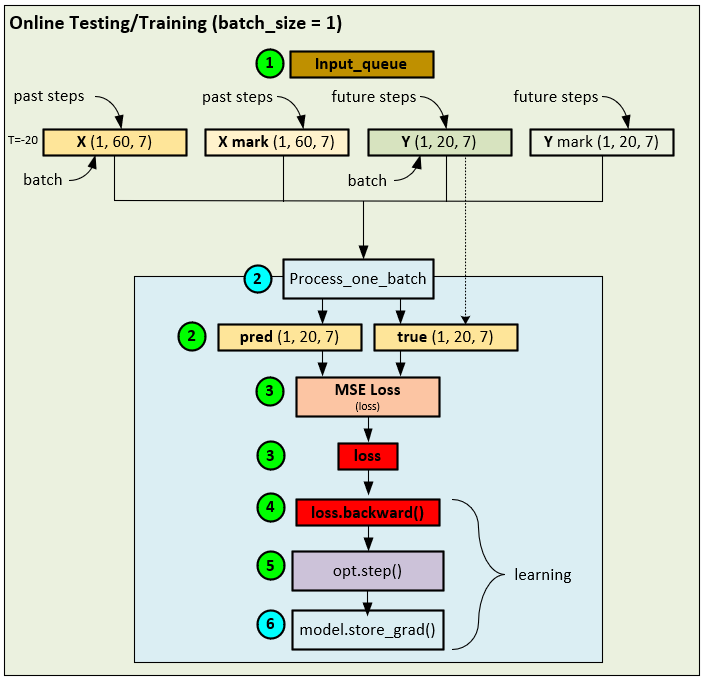
Online Testing/Training with Known Future Data
Once the batch-training is complete, the online training starts during the testing phase of the model. Unlike traditional models where testing does not alter the weights, the FSNet runs a single batch of inference followed by a single batch of online learning consisting of a backward pass and optimizer step.
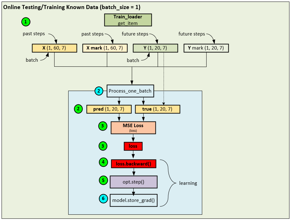
When running the online testing/training with known data, the following steps occur.
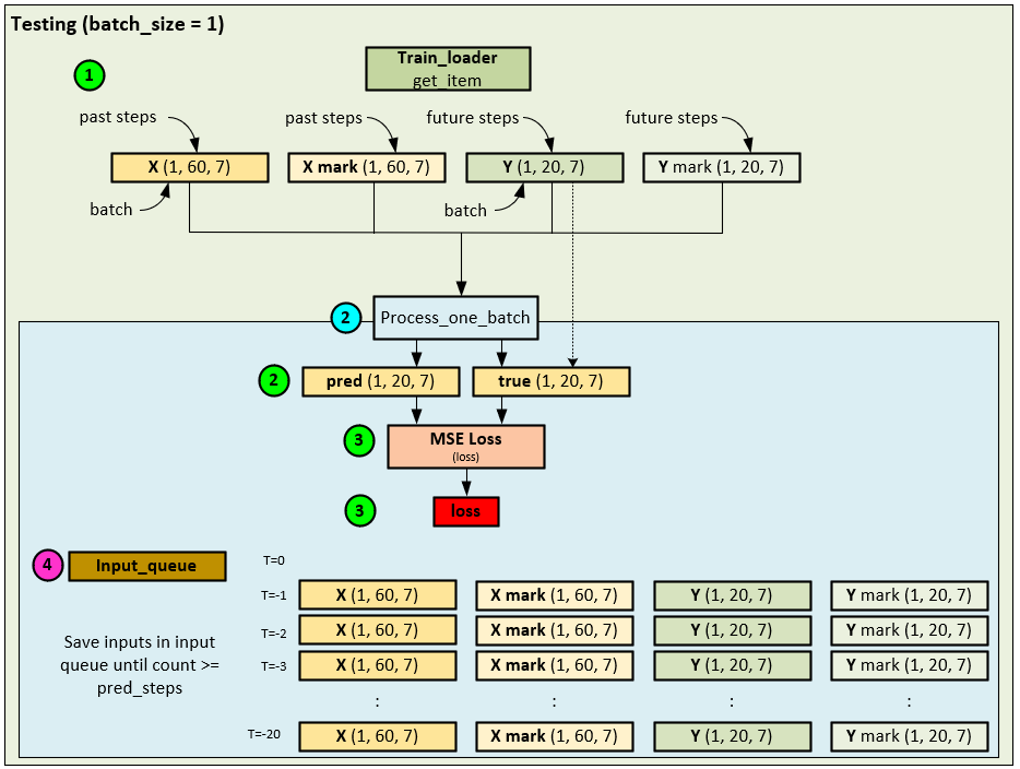
- Like batch training, a data loader is used to load each record from the dataset, but during testing the records are fed in sequence (e.g., not shuffled), and fed as a single batch size = 1.
- Next the single batch of data is sent to the Process_one_batch function which produces the pred and true tensors.
- Next, internal to the Process_one_batch function, the loss is calculated using the MSE Loss function.
- Next the loss if back propagated through the network, …
- …, and the final gradients from the single batch run are calculated and applied to the network – this is the online learning part of the network.
- And finally, the same model store_grad function is called to update a special convolution weight and determine whether to trigger the fast-learning update mechanism.
We have found this algorithm to work well when predicting one step into the future and have similar results to Liquid Neural Nets discussed in previous blog posts. In addition, online learning works well when predicting multiple future values but only seems to do so when the future targets are already known. Our tests run when future targets are not known struggled to show good results.
Results of Online Learning with Known Future Data
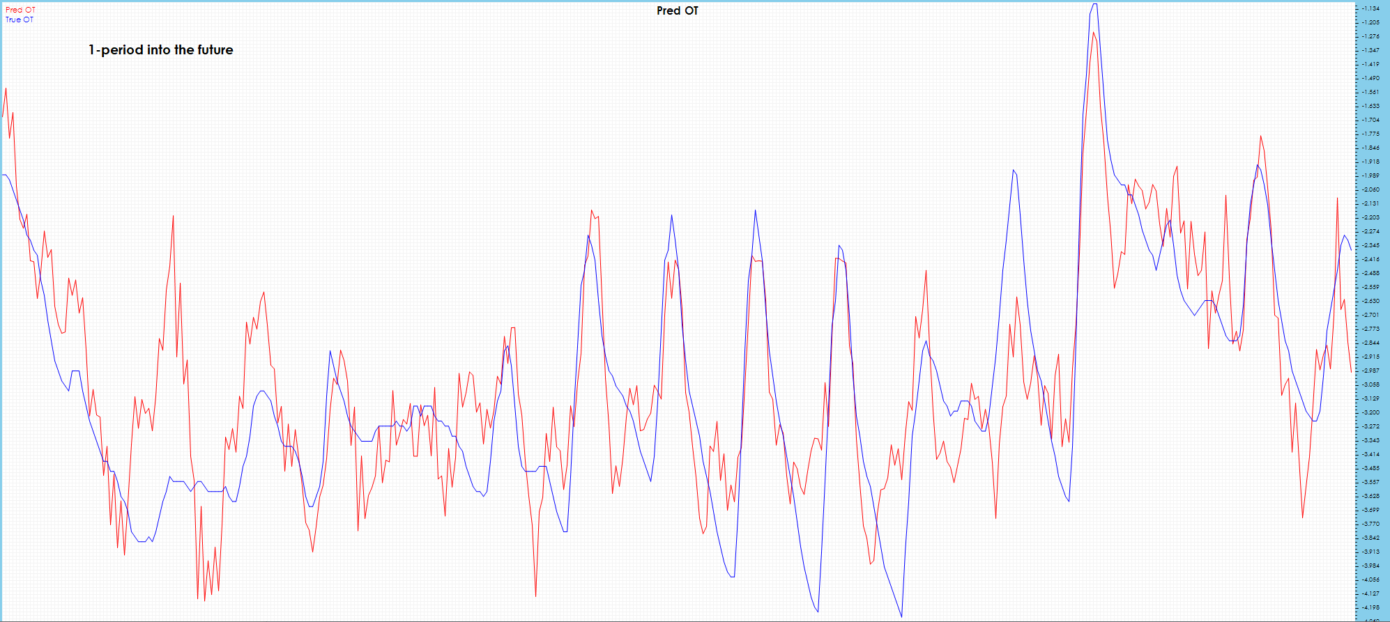
The following results are shown using the PyTorch FSNet GitHub project [3] by running the batch training for nearly 5 epochs of 87 steps each where early stopping occurs. Next, the online testing/training is run for 10781 iterations. The resulting NPY files are visualized using our own software. For these tests we will focus on the ETT HUFL and OT data fields and their predictions.
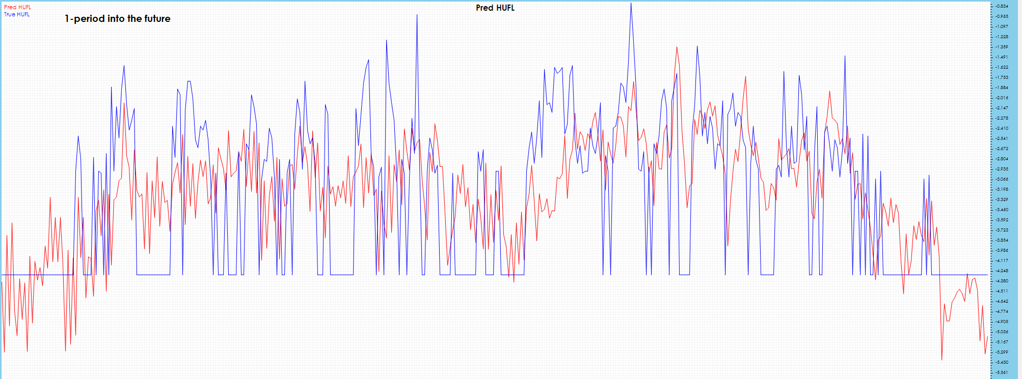
The online learning test with known data had a final MSE = 0.9597 and MAE = 0.5626
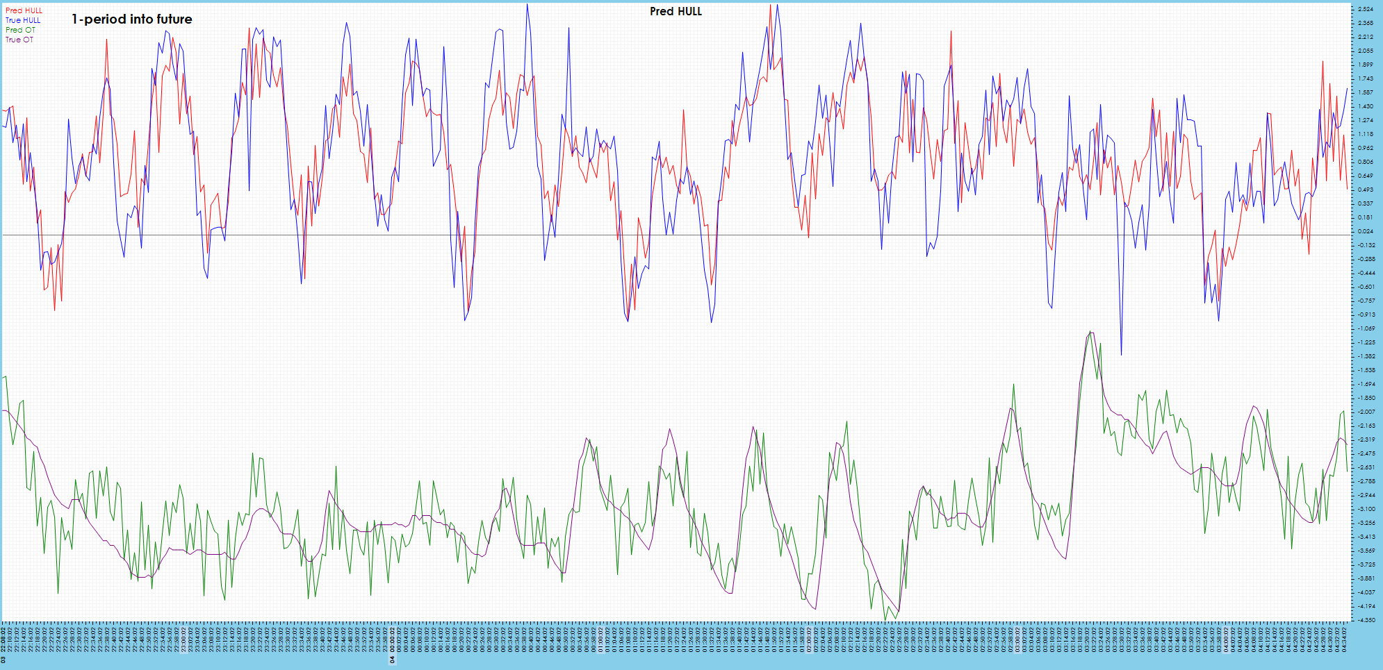
A single period into the future shows good tracking with the ground truth values.
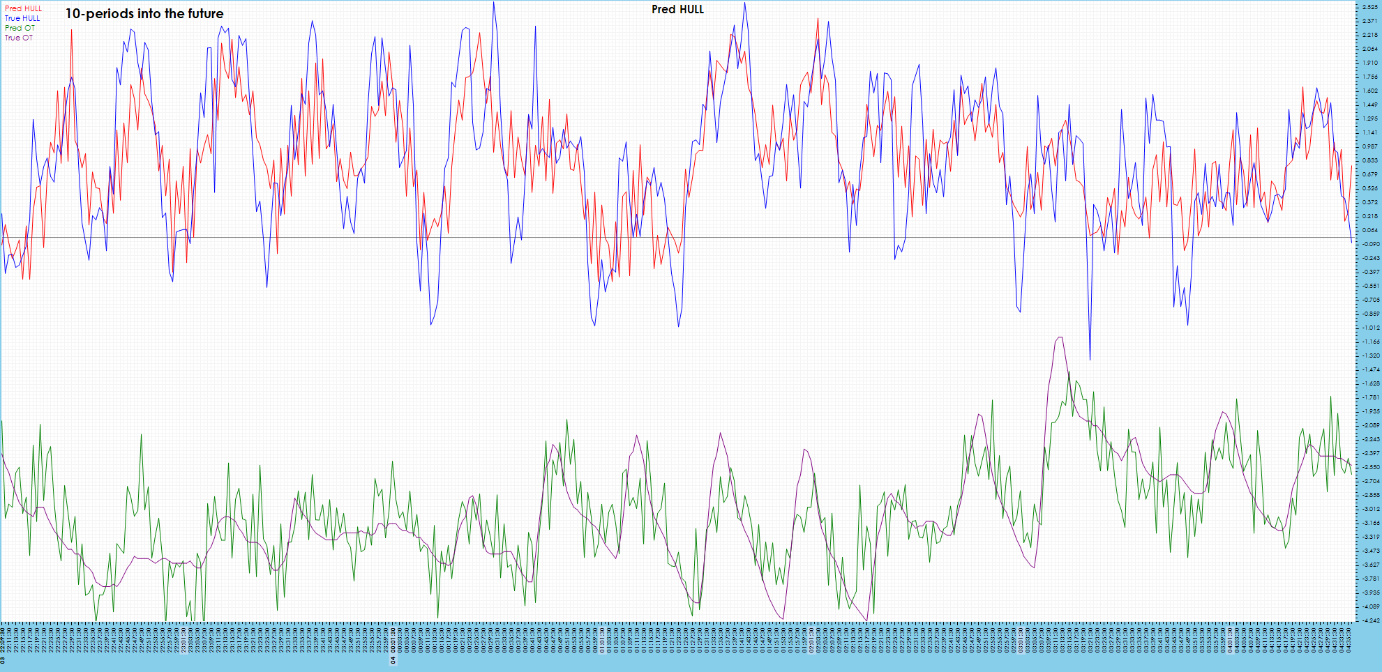
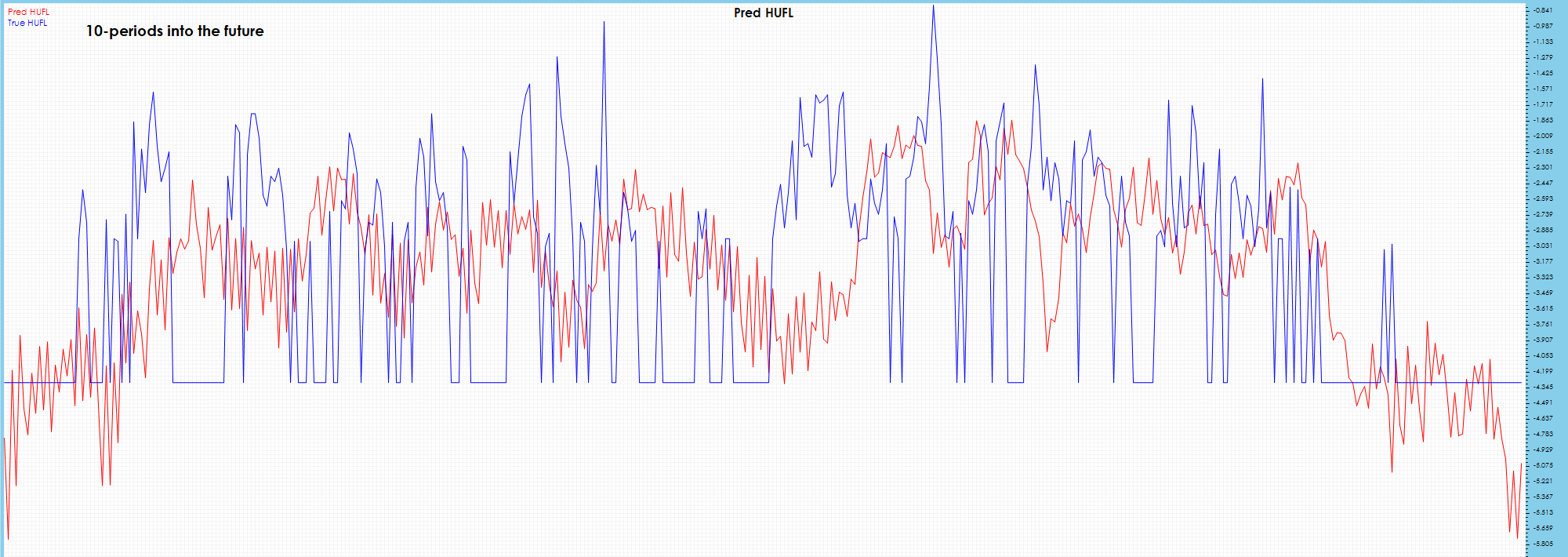
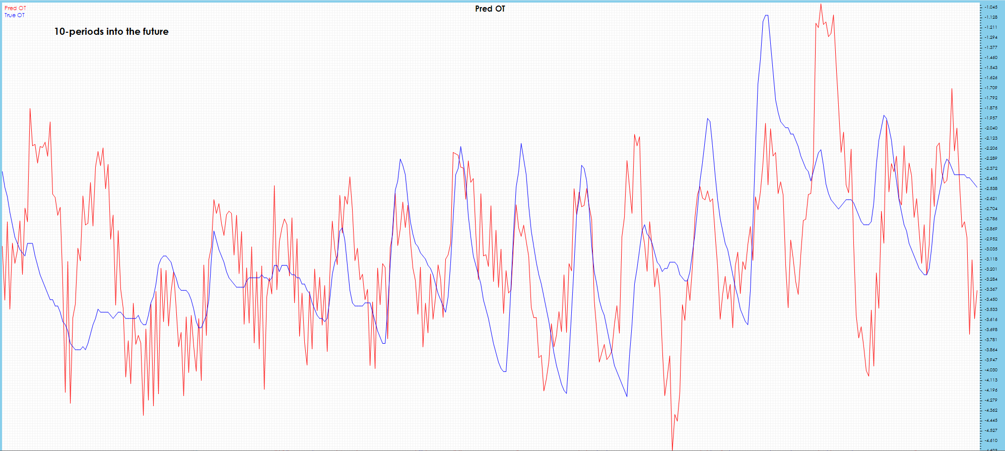
Some visible drift is shown in 10 periods into the future.
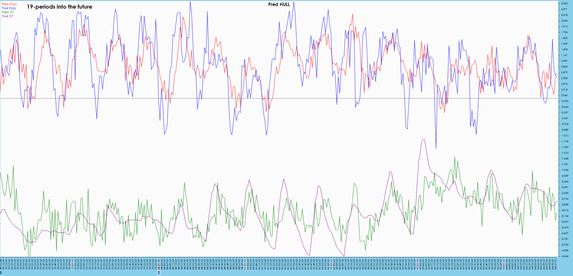
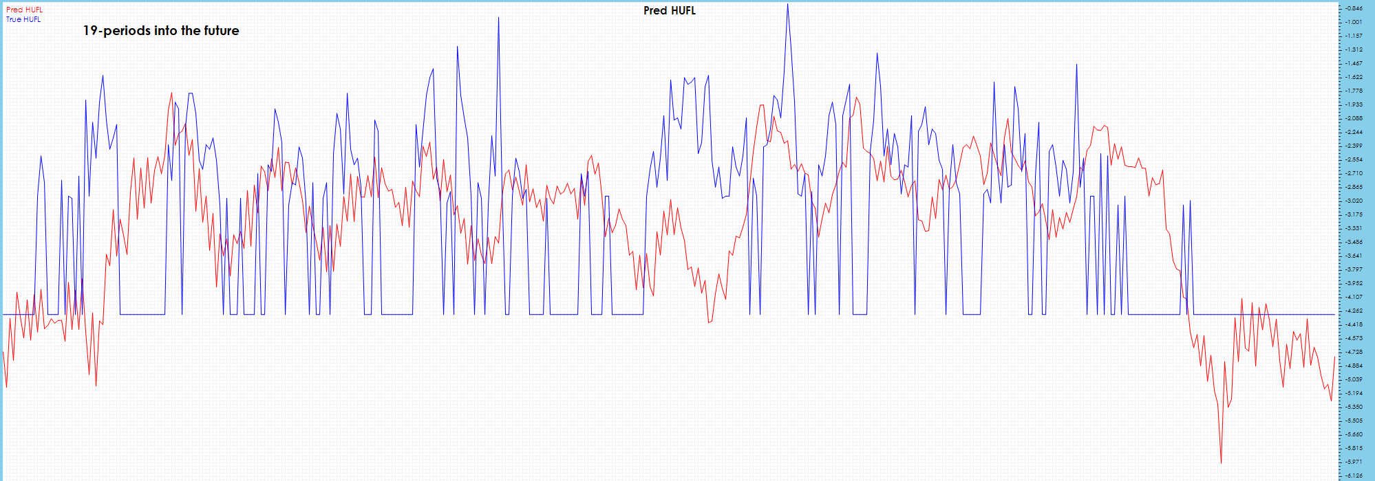
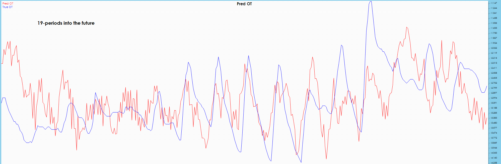
Visible drift starts to show in the predictions 19 periods into the future.
Online Training with Unknown Future Data – Buffered
To test the FSNet on unknown future values, we tested two alterations to the online training process. In the first process we buffered the input and target values, and only used them in training after they were 20 periods into the past or otherwise known.
When running the online testing/training with unknown future values, the following process was used.
- Data iteration was performed in sequence one single item at a time.
- The X, X mark and Y tensors were fed into the Process_one_batch function which only inferenced through the data to produce the pred and true
- Within the Process_one_batch function, the MSE Loss calculates the loss, but this loss is only used for reporting – no online learning occurs as we are only inferencing at this point.
- The input X, X mark and Y tensors are then stored in the input_queue to be used later in the online training as we cannot use the values at this stage for, we are predicting future values for which the ground truth values are not known yet.
Online Training with Buffered Data
Once the ground truth values within the input_queue are known (e.g., 20 steps after the present time) they are used for training.
The following steps occur when online training with the future ground truth values once they become known.
- The oldest item in the input_queue is removed as its ground truth values are now 20 steps into the past from the future and therefore known.
- The X, X mark and Y tensors are fed into the Process_one_batch function like before which first runs the inference to produce the pred tensor and the true tensor is created from the Y tensor.
- The MSE Loss is calculated using the pred and true tensors to create the loss value.
- The loss values are used to run the backward pass which propagates the error back through the network allowing for gradients to be calculated at each layer.
- The optimizer then calculates the final gradients and applies them to the learnable parameters of each layer.
As a final step, the special convolution weights are calculated and when appropriate, used to trigger the short-term updating mechanism.
Results of Online Learning with Unknown Future Data – Buffered
The following results are shown using the PyTorch FSNet GitHub project [3] by running the batch training for nearly 5 epochs of 87 steps each where early stopping occurs. Next, the online testing/training is run for 10781 iterations using the training method using the input_queue to ensure only training on known ground truth values. The resulting NPY files are visualized using our own software. For these tests we will focus on the same ETT HUFL and OT data fields and their predictions as before.
The online learning test with known data had a final MSE = 2.59 (vs 0.9597) and MAE = 0.7302 (vs. 0.5626) – not surprising, much worse than online learning with known ground truth values.
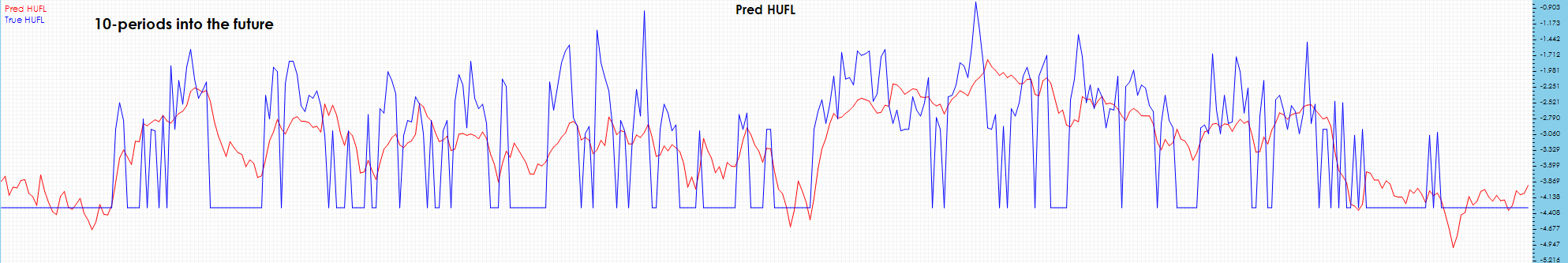
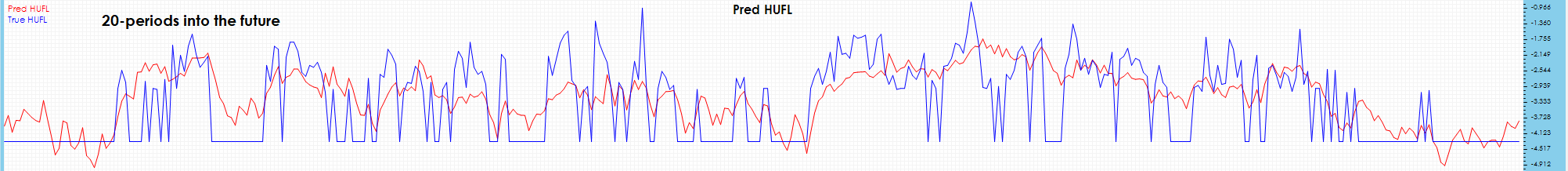
HUFL – Heavy Use Full Load
Predictions seem to catch the rough shape, but visibly do not catch most spikes.
Significant drift is visible on the 10-period chart.
Spikes are not predicted well and severe drift is visible on the 20-period prediction chart.
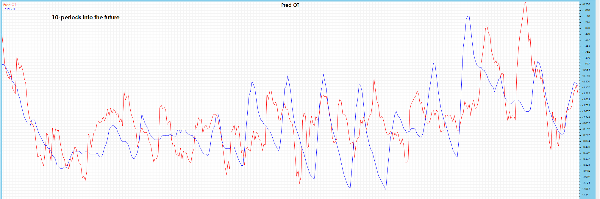
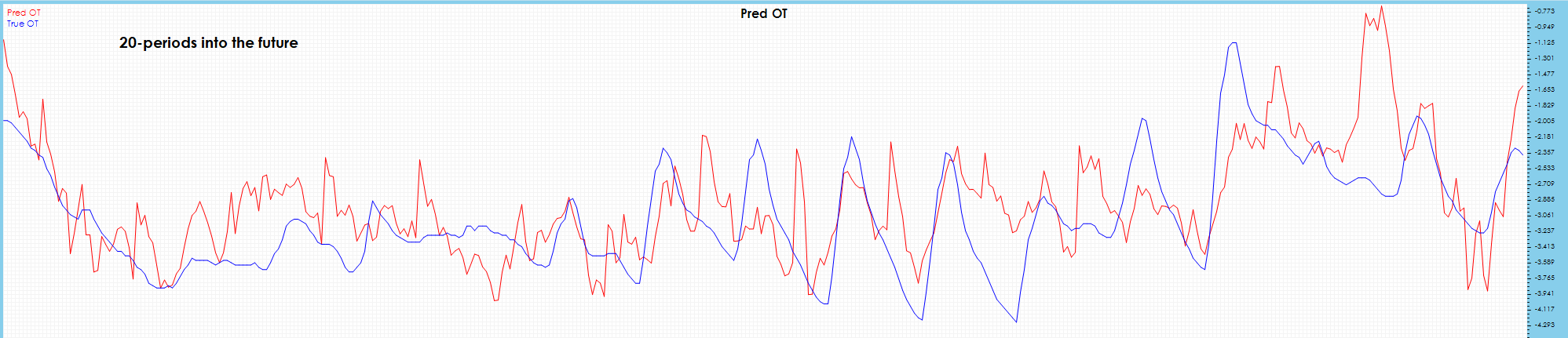
OT – Oil Temperature
Spikes are caught in 1-period future predictions, which look good and are similar to predictions that do not use the buffer.
In the 10-period future predictions, spikes are detected, but with much more jitter and severe drift observed in latter part of chart.
The 19-period prediction chart has somewhat less noise than 10 period, but severe drift observed in latter part of chart.
Online Training with Unknown Future Data – Generative
To test the FSNet on unknown future values, we tested a second method of prediction where we predicted only 1 future value with the same 60 input values. After running the online test/training for 8000 iterations to ‘train’ the model, we then iteratively ran inference over several steps into the future using each prediction as input for the next training cycle like the way a generative AI model runs.
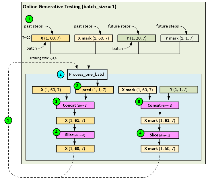
When using the online generative testing/training method the following steps occur.
- The data loader loads the tensors in sequence with a batch size = 1.
- Next, the X, X mark, and Y tensors are inferenced and online learned in a single learning step within the Process_one_batch function to produce the pred tensor of predictions 1 step into the future.
- The pred and input X tensors are then concatenated together, as are the Y mark and X mark
- The oldest step in the new X and X mark tensors are removed with a Slice operation producing the new X and X mark tensors containing the ground truth + 1 predicted future value.
- The new X and X mark tensors are then used as the new inputs.
Results of Online Learning with Unknown Future Data – Generative
The following results are shown using the PyTorch FSNet GitHub project [3] by running the model to only predict 1 period into the future. The batch training was run for nearly 5 epochs of 87 steps each where early stopping occurs. Next, the online testing/training is run for 8000 iterations using the standard testing/training method for online learning. After 8000 iterations, we ran the model forward 10 iterations and 20 iterations and, in each case, fed the predicted results back into the input to see how well the model predicted future values. The resulting NPY files are visualized using our own software. For these tests we will focus on the same ETT HUFL and OT data fields and their predictions as before.
The online generative learning test with known data had a final MSE = 0.6807 (vs 0.9597) and MAE = 0.4811 (vs. 0.5626) – but these do not consider our future predictions past 1 period.
HUFL – Heavy Use Full Load
Visually, the HUFL 10-period and 20-period future predictions seem to follow the trend but miss the larger peaks and valleys.
OT – Oil Temperature
Visually the 10-period and 20-period future predictions show severe drift across most peaks.
Results Summary
When using known target data or predicting one time period into the future, the FSNet appears to produce useful time-series predictions. However, given the observed drift and added jitter when predicting multiple, unknown future values we do not see using the FSNet for predicting more than one time period into the future.
FSNet Implementation Discussion
The main part of the FSNet implementation occurs within the Process_one_batch function as this function contains the overall model itself.
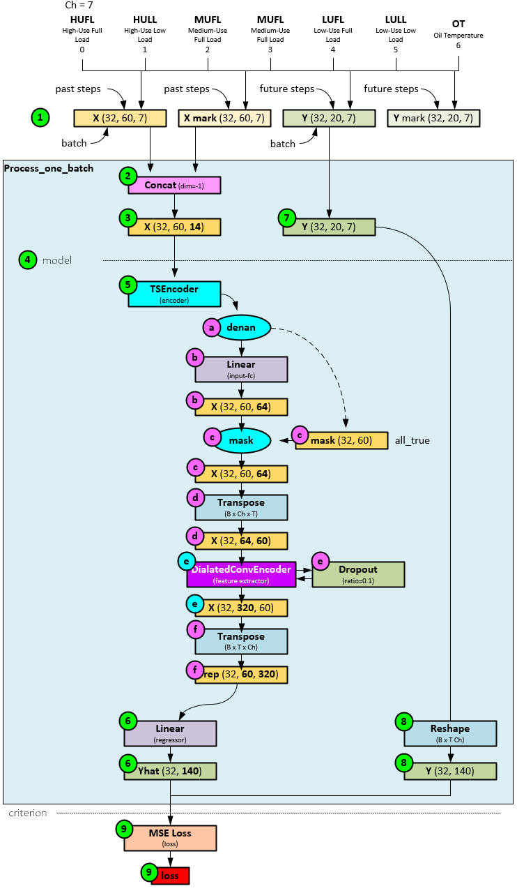
On each training or inference cycle, when this function is called, and the following steps occur.
- First the data loader loads the data into a full batch (when training) or single batch when testing/online training. During the data query, the X, X mark, Y and Y mark tensors are loaded where the X contains the input data, the X mark contains the input time data, the Y contains the target, and the Y mark contains the target time data.
- The X, X mark, Y and Y mark tensors are passed to the Process_one_batch function, which concatenates the X and X mark tensors…
- … to produce a new X tensor that has data + time included.
- Next, the model is run on the data.
- The model uses a TSEncoder layer to learn the temporal patterns within the data using numerous dilated convolution blocks – each with a progressively larger receptive field.
- When processing the X tensor, the TSEncoder first masks out all nan values if they exist.
- Next the denaned X tensor is passed through the fc input Linear layer which expands the 14-element channel to 64 items.
- If an external mask is supplied, it is applied to the Linear layer output. To produce the masked X
- The masked X tensor is transposed along the last two axes to swap the channel data with the time-step data axes, producing the transposed X
- The transposed X tensor is passed to the DialatedConvEncoder (discussed later), appropriate drop-out is applied, to produce the encoded X tensor.
- The encoded X tensor is re-transposed back to its original time-step, channel ordering, except now the channel data contains the 320-item encoding. Thew newly transposed encoded X tensor becomes the rep tensor.
- The rep tensor is passed through the regressor Linear layer to produce the 20 predictions, each containing 7 channel values for the predicted HUFL, HULL, MUFL, MULL, LUFL, LULL and OT values.
- The Y target values…
- … are reshaped to a shape like the Yhat predictions, …
- … and both are run through the MSE Loss to calculate the loss value.
DialatedConvEncoder Layer
The DialatedConvEncoder performs nearly all temporal pattern recognition using a set of dilated, specialized Convolution Blocks, each with a progressively larger receptive field.
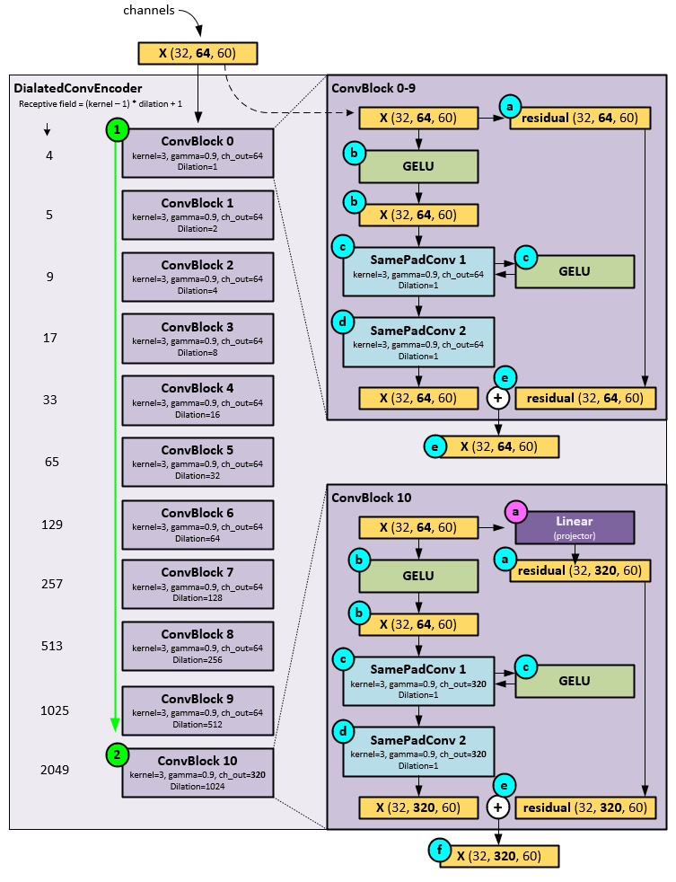
On each pass, the following steps occur within the DialatedConvEncoder Layer.
- The X tensor (which at this point is the transposed X tensor) is passed sequentially through a set of ConvBlocks where all but the last ConvBlock perform the same operations but with a progressively larger dilation setting.
- Upon receiving the X tensor, the ConvBlock first saves the X tensor as the residual tensor for use later.
- Next, the X tensor is run through a GELU activation layer.
- The resulting tensor is then sent to the first of two SamePadConv Layers (described later), and another GELU
- The resulting tensor is then sent to the second SamePadConv
- The resulting tensor from the second SamePadConv Layer is added to the residual tensor and passed along to the next ConvBlock.
- This process continues through all ConvBlocks util the last ConvBlock is reached. All previous ConvBlocks use the same channel_out size = 64, whereas the final ConvBlock uses a channel_out size = 320.
- In the last ConvBlock, the X tensor is passed through a Linear projection layer which expands the channels from 64 values to 320 values which becomes the new residual tensor.
- Next, the X tensor is run through a GELU activation layer.
- The resulting tensor is then sent to the first of two SamePadConv Layers with channel_out = 320, and another GELU
- The resulting tensor is then sent to the second SamePadConv Layer with channel_out = 320.
- The resulting tensor from the second SamePadConv Layer is added to the residual tensor and passed along as the output of the DialatedConvEncoder
SamePadConv Layer
Each SamePadConv Layer performs both the slow and fast learning at a specific dilation setting (e.g., covering a certain receptive field).
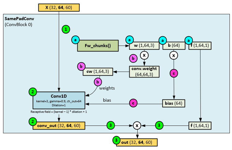
When running through each of the SamePadConv Layers, the following steps occur.
- The X tensor from the ConvBlock is passed to the SamePadConv
- Before processing the X tensor, the fw_chunks function (described layer) is run to produce the w, b, and f learnable parameters.
- The w parameter is multiplied by the Conv1D weights to produce the new Conv1D weights (cw).
- And the b parameter is multiplied by the bias parameter to produce the new Conv1D bias (bias).
- With the new weights and bias, the X tensor is run through the Conv1D Layer with its specific dilation setting to produce the conv_out
- The conv_out tensor is then multiplied by the f learnable parameter produced by the fw_chunks function to produce the out
This process is where ‘slow’ learning occurs, whereas within the fw_chunks function the ‘fast’ learning occurs.
fw_chunks function
The fw_chunks function runs in two modes: a normal mode where Linear layers are used to produce the w, b and f parameters, and a triggered mode where the w, b and f parameters are updated with the ‘fast’ learning using the memory (stored in W tensor) that is adapted through attention applied to a concatenation of w, b and f, and the W tensor used as a short-term memory.
First, we describe the normal mode.
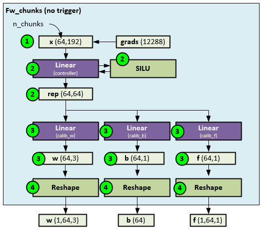
When run in the normal, non-triggered mode, the fw_chunks performs the following steps.
- First the internal gradients stored in the grads tensor are copied to the x tensor and reshaped to several chunks.
- The reshaped x tensor is fed through the controller which consists of a Linear layer and SILU activation layer to produce the rep
- The rep tensor is then fed into three separate Linear layers each used to calibrate the w, b, and f parameters respectively.
- The w, b and f outputs are reshaped and sent out as the new w, b, and f
Given that the w, b, and f parameters are later used in the SamePadConv layer as the Conv1D weight, bias and output scale, these learnable parameters retain the ‘slow’ learning of the model at each ConvBlock for each receptive field defined by the dilation setting.
When running the fw_chunks function in a triggered mode, things get a little more complicated – this is where the ‘fast’ learning occurs.
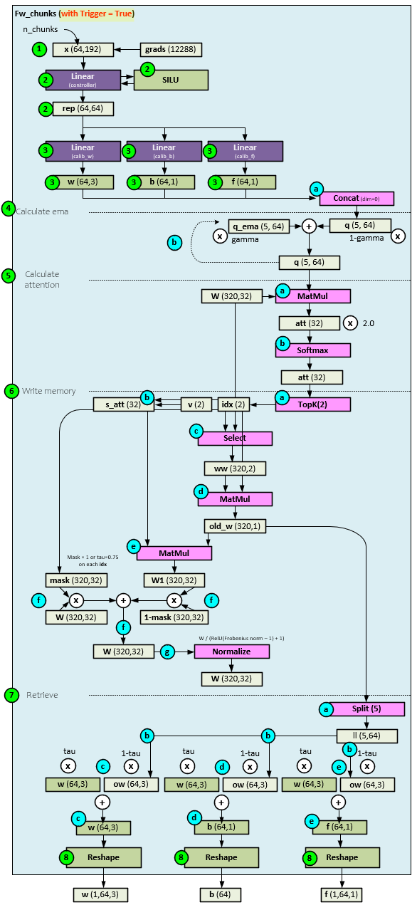
When run in a triggered mode, the fw_chunks function takes the following steps.
- First the internal gradients stored in the grads tensor are copied to the x tensor and reshaped to several chunks.
- The reshaped x tensor is fed through the controller which consists of a Linear layer and SILU activation layer to produce the rep
- The rep tensor is then fed into three separate Linear layers each used to calibrate the w, b, and f parameters respectively.
- Up until this point the fw_chunks function has performed the same steps as the non-triggered mode, but this is where things change. First the Q ema is calculated.
- Instead of the w, b and f sent out as outputs, these values are instead concatenated together to produce a new q
- The new q tensor is smoothed with an ema by adding a portion of the q tensor to a portion of the previous q_ema tensor to produce a new q tensor that also becomes the new q_ema tensor for the next cycle. The gamma hyperparameter controls the amount of q used in this ema.
- Next the q tensor is used to calculate the attention between the q tensor and the W memory parameter used for short term fast learning storage.
- The attention is calculated by performing a MatMul on q and W to produce the new att
- The att tensor is run through a Softmax to find the attention values.
- Next the memory is written (e.g., the W parameter is updated) [1] (page 5).
- The first step in updating the W parameter is to select the top att attention values and their indexes which become the v and idx
- A new s_att tensor is created with the same size as att but set to all zeros except in the two indexes of idx where the values of v are placed.
- Next, the values of W at the indexes of idx are selected and placed in the ww tensor, thus selecting the most important parts of W that should have the most attention.
- A MatMul is performed on the ww and idx tensors to produce the old_w
- And another MatMul is performed on the old_w and the s_att tensor to produce a new W1 parameter, held locally.
- A mask tensor is created with the same size as W and filled with all 1’s except on the indexes of idx where they are filled with a value of tau (default = 0.75). The W parameter is updated by multiplying the current W with the mask and adding to the local W1 parameter multiplied by the inverted mask (1-mask).
- The new W parameter is normalized by dividing by the RELU(Frobenius Norm of W – 1) + 1.
- Next the new w, b and f values are calculated using the old_w tensor calculated in step 6.e, above.
- In the first step the old_w tensor is split into five pieces.
- The first three pieces become the ow tensor, the next piece becomes the ob tensor, and the last piece becomes the of
- Using tau, a new w is calculated by taking tau of the existing w and adding that to 1-tau of the new ow
- Using tau, a new b is calculated by taking tau of the existing b and adding that to 1-tau of the new ob
- Using tau, a new f is calculated by taking tau of the existing f and adding that to 1-tau of the new of
- The new w, b, and f tensors are reshaped and returned as the new values.
What Causes the Trigger?
The store_grad function called at the end of each learning pass, just after the optimizer step, sets the trigger in each layer using the following logic. Each SamePadConv layer implements the store_grad function.
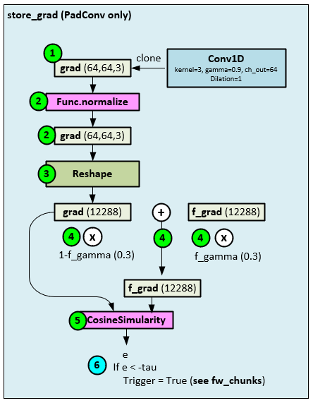
The following steps occur when the store_grad function is called.
- First the gradients from the Conv1D layer are cloned to the grad
- Next, the grad values are normalized, …
- …, and reshaped (flattened).
- The flattened grad values are multiplied by (1-f_gamma) and added to the previous f_grad values multiplied by f_gamma to produce the updated f_grad
- A CosineSimilarity is run on the grad and f_grad values to produce e. Since updating the memory W is expensive the trigger is only set “when a substation representation change happens.” [1] To detect such a change two EMA’s are calculated with differing coefficient sizes (e.g., one coefficient gamma for grad and a smaller coefficient f_gamma for f_grad).
- When the cosine similarity e is < -tau [1] (page 5), the memory update is triggered for W.
Summary
In summary, the FSNet looks like a great candidate model for online learning when predicting one period into the future. We have not yet compared the FSNet to the performance of the Liquid Neural Network when using online learning but see some similarities in their overall performance.
Happy Deep Learning with Time Series!
[1] Learning Fast and Slow for Online Time Series Forecasting, by Quang Pham, Chenghao Liu, Doyen Sahoo, and Steven C.H. Hoi, 2022, arXiv:2202.11672
[2] GitHub: zhouhaoyi/ETDataset, by zhouhaoyi, 2021, GitHub
[3] GitHub: salesforce/fsnet, by Salesforce, 2022, GitHub