

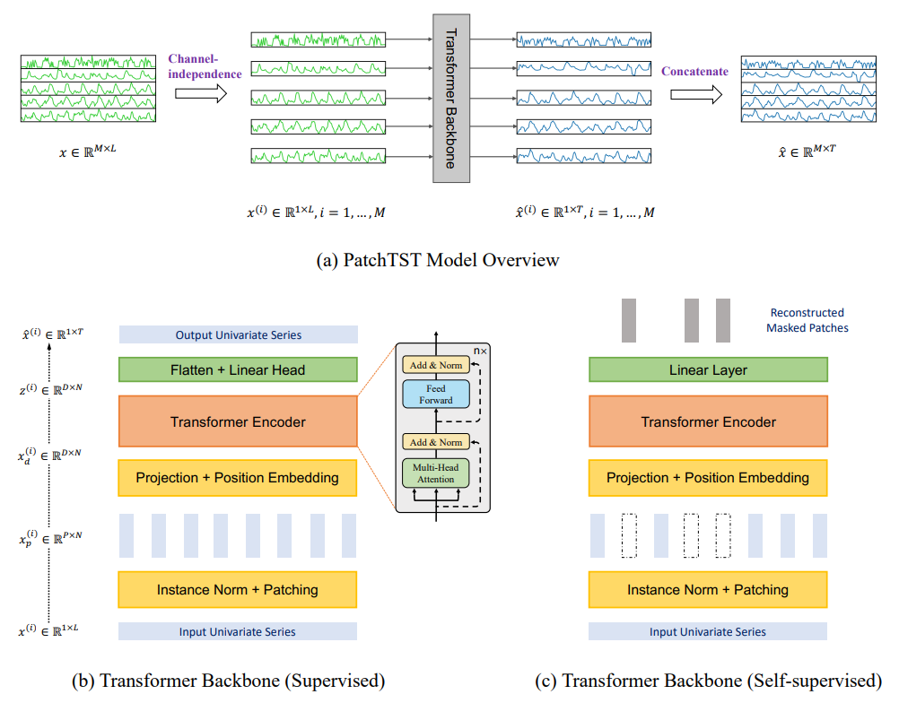
In this blog post, we evaluate from a programmer’s perspective, the PatchTST model described in “A Time Series is Worth 64 Words: Long-term Forecasting with Transformers” by Nie, et. al., 2022. The PatchTST is a transformer-based model for multivariate time-series prediction that separates the input data into ‘patches’ that are then fed into a standard transformer-based architecture. The patching design has three benefits: “local semantic information is retained in the embedding; computation and memory usage of attention maps are quadratically reduced given the same look-back window; and the model can attend longer history.” [1]
Data Processing
For comparison purposes, we use the same ETTh2 electricity dataset as was used in the FSNet model discussion in our previous post, with a sequence length of 60, predicted length of 20 and label length of zero. As displayed below, you will notice that the data processing used for the PatchTST model is very similar to that used with the FSNet but with a small difference in the normalization of the time variable X mark, which are pre-normalized in the PatchTST model, but as you will see later, are not even used by the model.
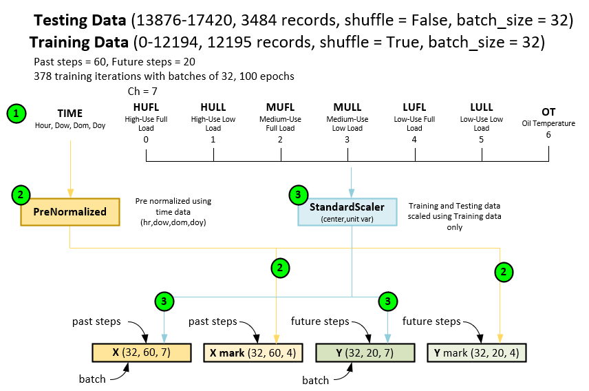
During data processing for the PatchTST, the following steps occur.
- First the dataset is loaded with the time + 7 fields per record.
- The time field is pre normalized when loaded to produce the X mark and Y mark tensors.
- Next, the other 7 data fields are fitted to a StandardScaler with the training data then scaled across both the training and testing data. Note, the StandardScaler performs data centering with a unit variance. The fit values are placed in the X input and Y target data tensors. These tensors are fed into both the training and testing cycles.
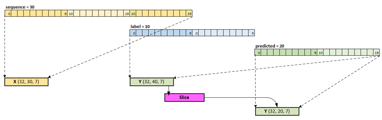
A Note on Label Length
As noted by freak11 on StackOverflow, “The machine learning model is trained on the label length. The label length refers to the number of timesteps in the future for which the ground truth values are available during training. In other words, the model is trained to predict the values of the time series at time steps that fall within the label length given the values of the previous time steps. The prediction length, on the other hand, specifies the number of timesteps in the future for which the model is asked to make predictions during inference after the training is completed.” [2]
However, when looking closely at how the label is used when building the batches [3] of data, we see that the label includes data both in the sequence and predicted areas, which are then sliced off during the loss calculation [3].
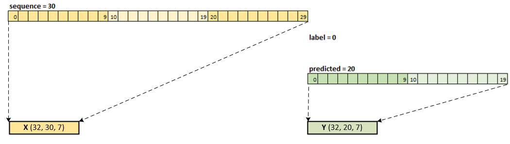
To make a similar comparison to the FSNet online training, we have set the label = 0 to produce the following loading for input X and target Y.
Training Process
The training process uses a standard batch processing forward pass coupled with a loss calculation using the MSE Loss that is then fed through the backward pass to calculate the gradients that are then applied using an Adam optimizer. A batch size = 32 is used during the initial training process.
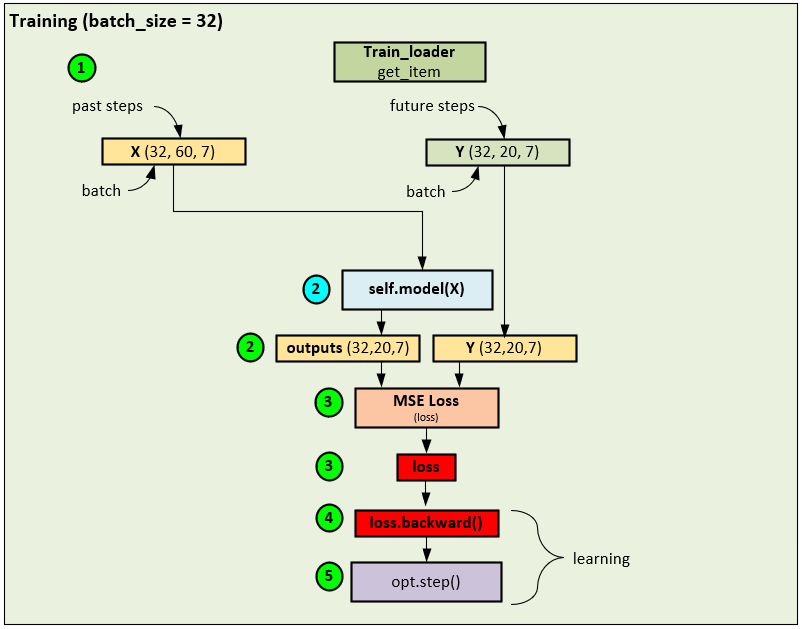
During the training phase, the following steps occur.
- A data loader is used to collect shuffled data records to build each batch of 32 that make up the input X, and target Y tensors. Note, 60 past steps are used in the X input data and 20 future steps are used in the Y targets where the X and Y tensors contain the 7 input fields (HUFL, HULL, MUFL, MULL, LUFL, LULL and OT). The X mark and Y mark tensors are filled with 4 fields related to the current time of the record which include the Hour, Day of Week, Day of Month, and Day of Year. However, the time tensors are not used when training the PatchTST model.[3]
- The input X tensor is fed into self.model() which runs the model to produce the predicted outputs.
- The output and Y (target) tensors are fed into the MSE Loss to calculate the loss value.
- And the loss value is used to run the backward pass that propagates the error back through the network and calculate the gradients at each layer.
- An Adam optimizer is used to calculate and apply the final gradients to the weights of each trainable parameter.
This standard batch training is used to train the network over 100 epochs of 378 iterations each.
Prediction Results
The following results are shown using the PyTorch PatchTST GitHub project [3] by running the batch training for over 30 epochs of 378 steps each where early stopping occurs. The resulting NPY files are visualized using our own software. For these tests we will focus on the ETT HUFL and OT data fields and their predictions.
The batch training final MSE = 0.1101 and MAE = 0.2229. These results are notably better than the MSE = 0.9597 and MAE = 0.5626 observed in the FSNet tests but note the PatchTST ran for many more epochs (over 30 vs 6) during batch training. However, PatchTST does not do any online learning like the FSNet.
HUFL – High Use Full Load
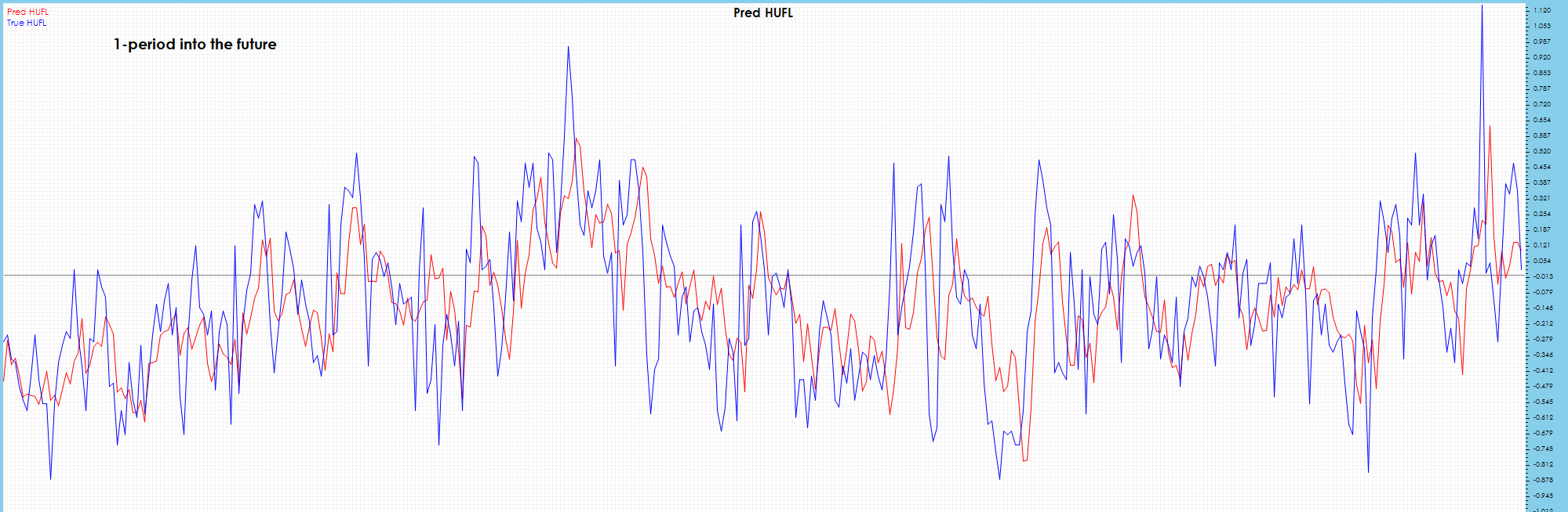
The HUFL one-period future predictions match the target values well and appear to catch most major peaks and valleys.
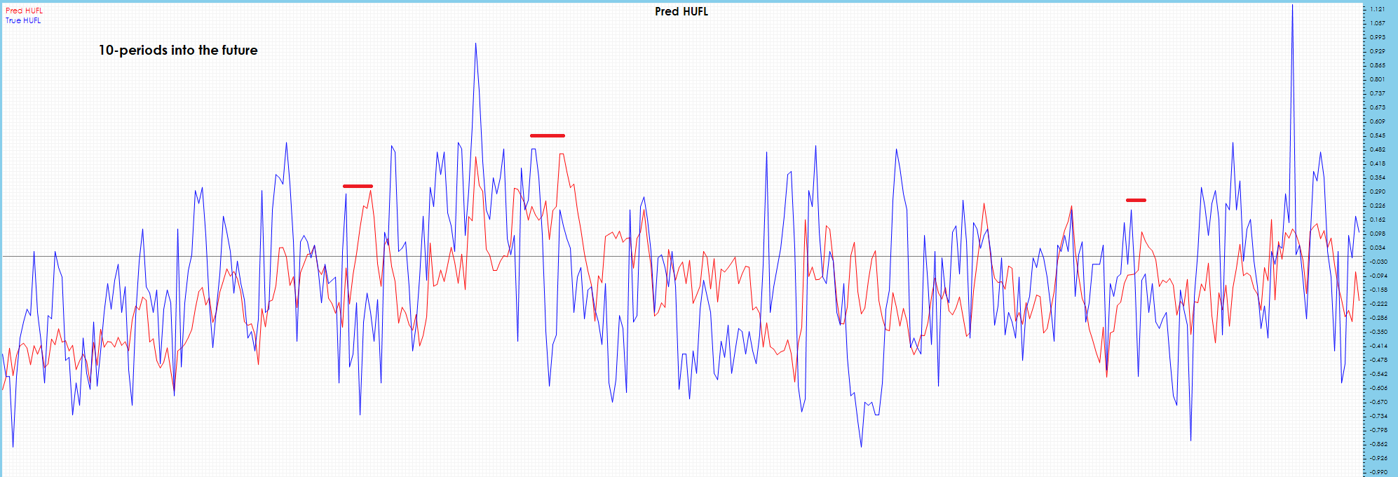
The HUFL 10-period future predictions appear to have some visible drift.
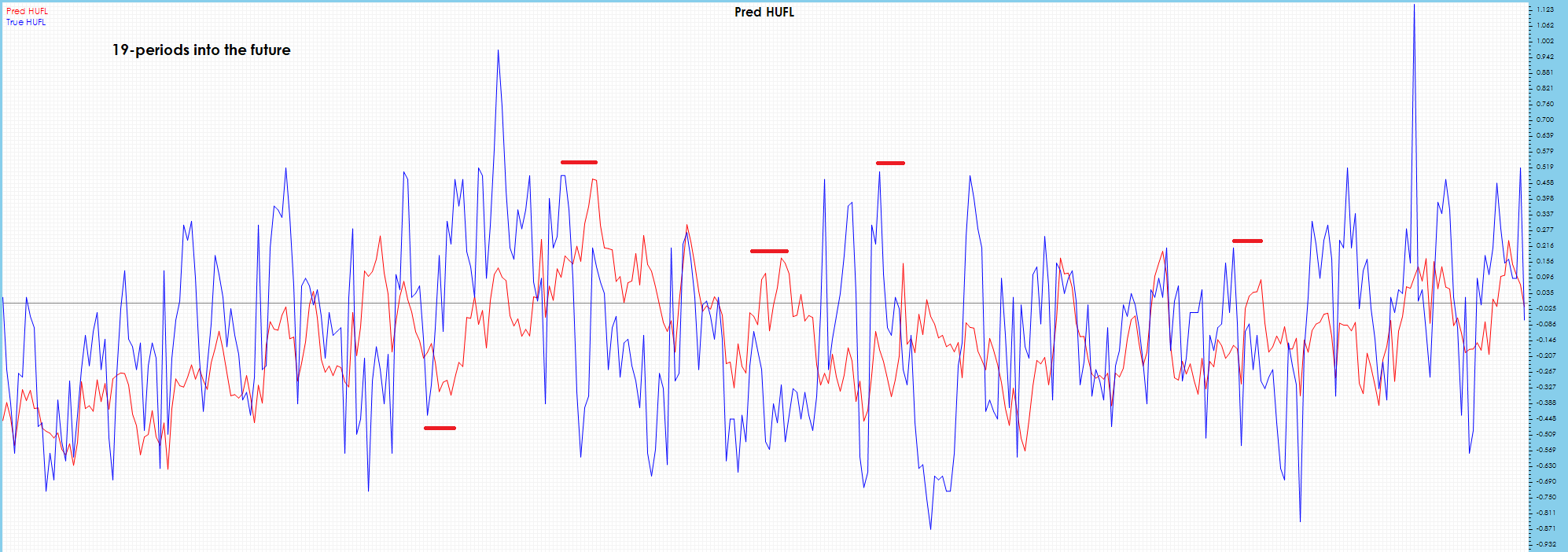
More visible drift shows up in the HUFL 19-period future predictions.
OT – Oil Temperature
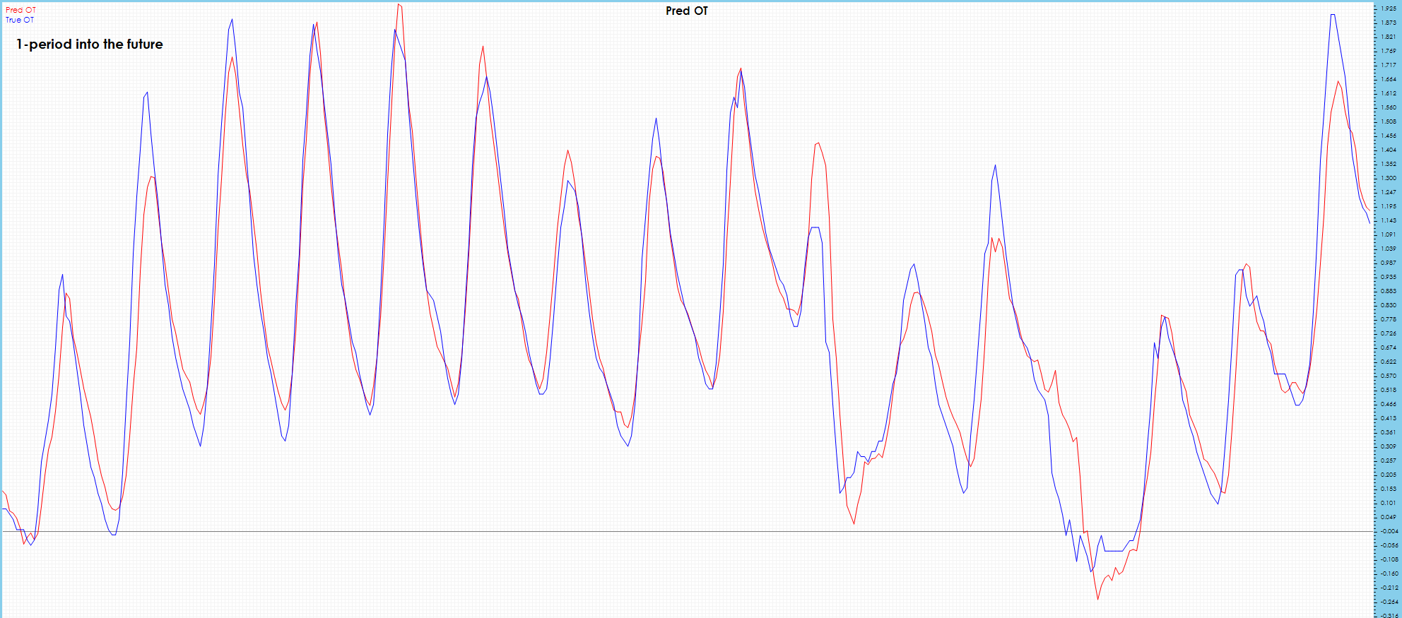
As expected, the OT 1-period future predictions are very good and match the targets very well.
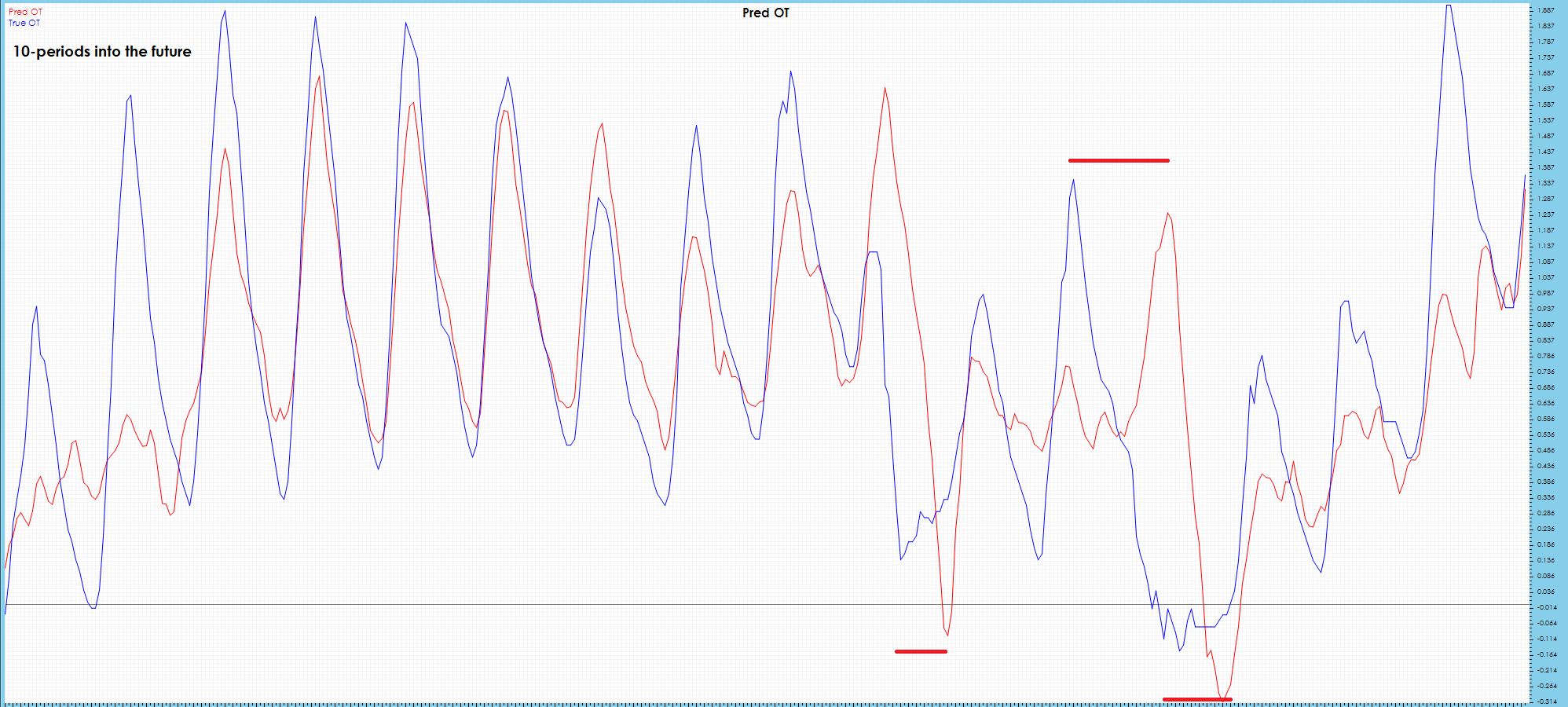
Some drift is visibly observed in the OT 10-period future predictions.
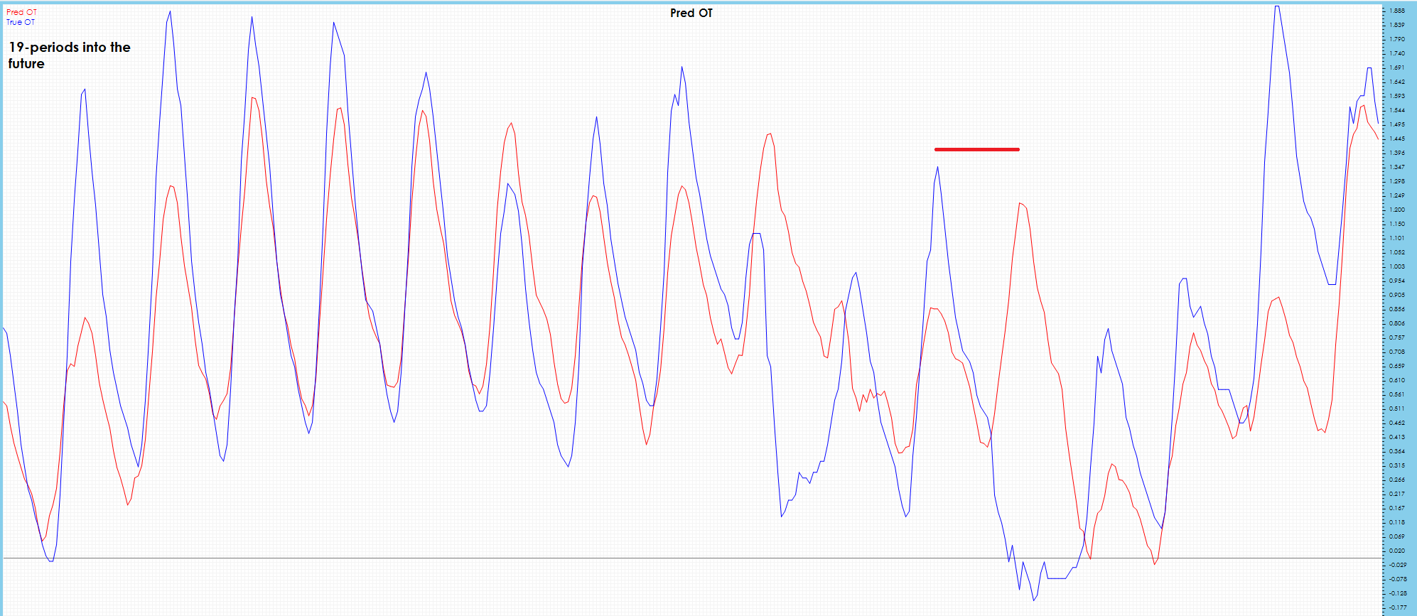
Surprisingly, the OT 19-period future predictions appear to have less drift than the OT 10-period future predictions.
PatchTST Implementation Discussion
There are two different modes of training supported by the PatchTST model: a normal mode and a decomposition mode that learns short term patterns in the data along with more long-term trend data calculated with a moving average.
Normal Model Mode
When running in the normal mode, the main workhorse of the model is the PatchTSTBackbone layer.
The following steps occur when running the normal model mode.
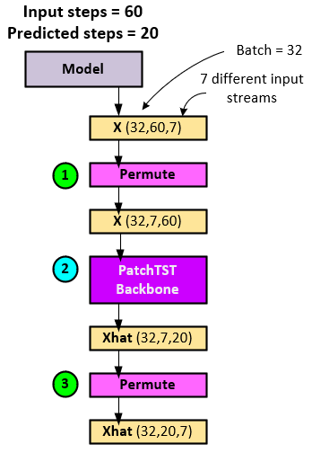
- The X input tensor is permuted, swapping the steps and channel axes (last two axes). Note the input X tensor has 60 input steps.
- The permuted X tensor is fed into the PatchTSTBackbone layer which performs the transformer-based model operations to produce the predictions in the Xhat
- The Xhat tensor is permuted back to its Batch x Steps x Channel shape. Note the Xhat predictions have 20 predicted future steps.
Decomposition Model Mode
The decomposition model mode is like the normal mode but first calculates the residual and trend from the X tensor data then runs a PatchTSTBackbone layer on each, adding the two results to form the final Xhat tensor containing the predictions.
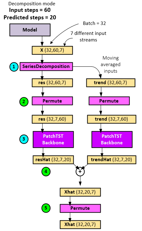
When running the decomposition model mode, the following steps occur.
- The X input tensor is fed into the SeriesDecomposition layer which calculates a moving average across each of the input channels within the X tensor to produce new res (residual) and trend tensors.
- Both res and trend tensors are permuted, swapping the steps and channel axes (last two axes). Note both tensors have 60 input steps.
- The permuted res tensor is fed into a PatchTSTBackbone layer which performs the transformer-based model operations to produce the predictions placed in the resHat and the permuted trend tensor is fed into a secondary PatchTSTBackbone layer which performs the transformer-based model operations to produce the trend predictions placed in the trendHat tensor. Note these two independent operations could easily run in parallel on two separate GPUs.
- Next, the resHat and trendHat tensors are added together to produce the Xhat
- As a final step, the Xhat tensor is permuted to swap the last two axes so that the final Xhat tensor has the ordering Batch x (predicted) Steps x Channel.
PatchTSTBackbone Layer
The PatchTSTBackbone Layer is the main workhorse of the PatchTST model that takes care of creating the patches and running them through the transformer-based model.
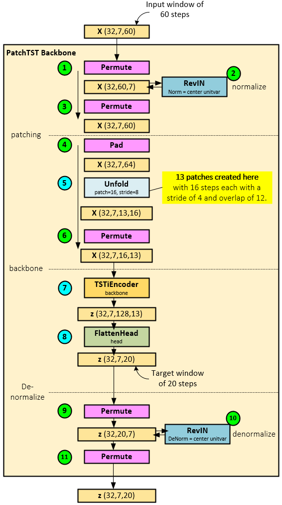
The following steps occur when running the PatchTSTBackbone Layer.
Normalization
- First the X tensor is permuted back to the Batch x Steps x Channel ordering.
- The permuted X tensor is then sent to the RevIN [4][5] layer that essentially normalizes the data by centering each channel and transforming each to a unit variance with affine learning. “Statistical properties such as mean and variance often change over time in time series, i.e., time-series data suffer from a distribution shift problem. This change in temporal distribution is one of the main challenges that prevent accurate time-series forecasting. To address this issue, we propose a simple yet effective normalization method called reversible instance normalization (RevIN), a generally-applicable normalization-and-denormalization method with learnable affine transformation.”[4][5]
- The normalized X tensor is then permuted back to the Batch x Channel x Steps ordering. Note, steps 1-3 are optional and may not be necessary when working with data already scaled using the StandardScaler, noted in the data processing section above.
Patching
- During patch creation, the normalized X tensor is first padded to allow for creating equally sized patches.
- An Unfold layer is used to create 13 patches (number of patches depends on sequence length and patch size), each with 16 steps and separated with a 4-step stride thus causing a 12-step overlap. After patching, the patch tensor has the shape Batch x Channel x Patch x Patch Data and looks as follows.
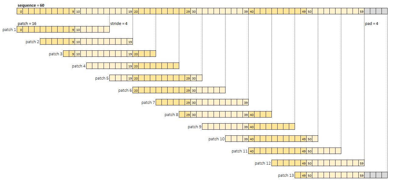
- The patch tensor is permuted to the shape Batch x Channel x Patch Data x Patch.
Backbone
- Next, the permuted patch tensor is fed into the TSTiEncoder backbone layer which produces the z tensor of shape Batch x Channel x Transformer Prediction Data x Patch.
- A FlattenHead layer is used to learn the final predictions from the z tensor which are output in the shape Batch x Channel x Prediction Steps, where there are 20 prediction steps.
De-Normalization
- Lastly, if normalization was performed during steps 1-3, a de-normalization occurs where the predicted values in the z tensor are permuted to the shape Batch x Prediction Steps x Channel.
- The permuted z tensor is the run through the RevIN[4][5] layer to de-normalize the data, …
- … and permuted back to the Batch x Channel x Prediction Steps shape.
FlattenHead Layer
Even though the FlattenedHead layer occurs after the TSTIEncoder Layer, we discuss it here for the TSTIEncoder Layer has a detailed chain of discussion.
The main goal of the FlattenHead layer is to provide the final processing that transforms the Transformer Data predictions into the final predicted step values.
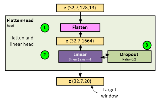
The following steps occur when running the FlattenHead Layer.
- First the z tensor is flattened along its last two axes converting the shape from Batch x Channel x Transformer Data x Patch to Batch x Channel x Transformer Data * Patch.
- The flattened z tensor is run though a Linear layer to produce the predicted future steps.
- The Linear layer output is run through a final Dropout layer to produce the final outputs.
TSTiEncoder Layer
The TSTiEncoder Layer projects the inputs, adds position data to it and passes the data to the TSEncoder for transformer processing.
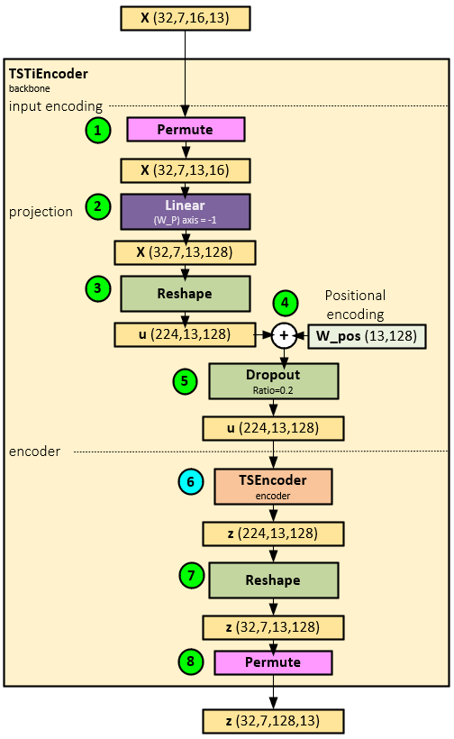
When running the TSTiEncoder Layer, the following steps occur.
- The X tensor is first permuted, swapping the last two axes to form the shape Batch x Channel x Patch x Patch Data.
- A Linear layer is used to project the patch data.
- The projected patch data is reshaped into the u tensor which has the Batch and Channel combined for a new shape of Batch * Channel x Patch x Patch Data.
- Position (temporal) data from the W_pos tensor is added to the reshaped u tensor (which explains why the X mark tensor is not used), …
- … and passed through a Dropout layer, …
- … and then to the TSEncoder layer for transformer encoding which outputs the z tensor with shape Batch * Channel x Patch x Transformer Encoding.
- The z tensor is reshaped to separate the Batch and Channel for a new shape of Batch x Channel x Patch x Transformer Encoding.
- The reshaped z tensor is then permuted to a final shape of Batch x Channel x Transformer Encoding x Patch.
TSEncoder Layer
The TSEncoder layer essentially runs the transformer blocks in sequence to produce the transformer encodings.
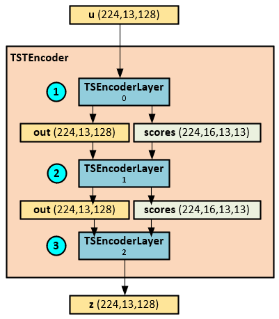
The following steps occur when running the TSEncoder Layer.
- The u input tensor is sent to a sequence of TSEncoderLayer layers depending on the n_layers configuration setting.
- Each TSEncoderLayer outputs the out and attention scores tensors which are both passed to the next TSEncoderLayer in sequence.
- The final TSEncoderLayer outputs the final out tensor as the z tensor.
TSEncoderLayer (Transformer Block) Layer
The TSTEncoderLayer performs the transformer block processing that combines multi-head attention with the Add & Norm and Position-wise FF processing.
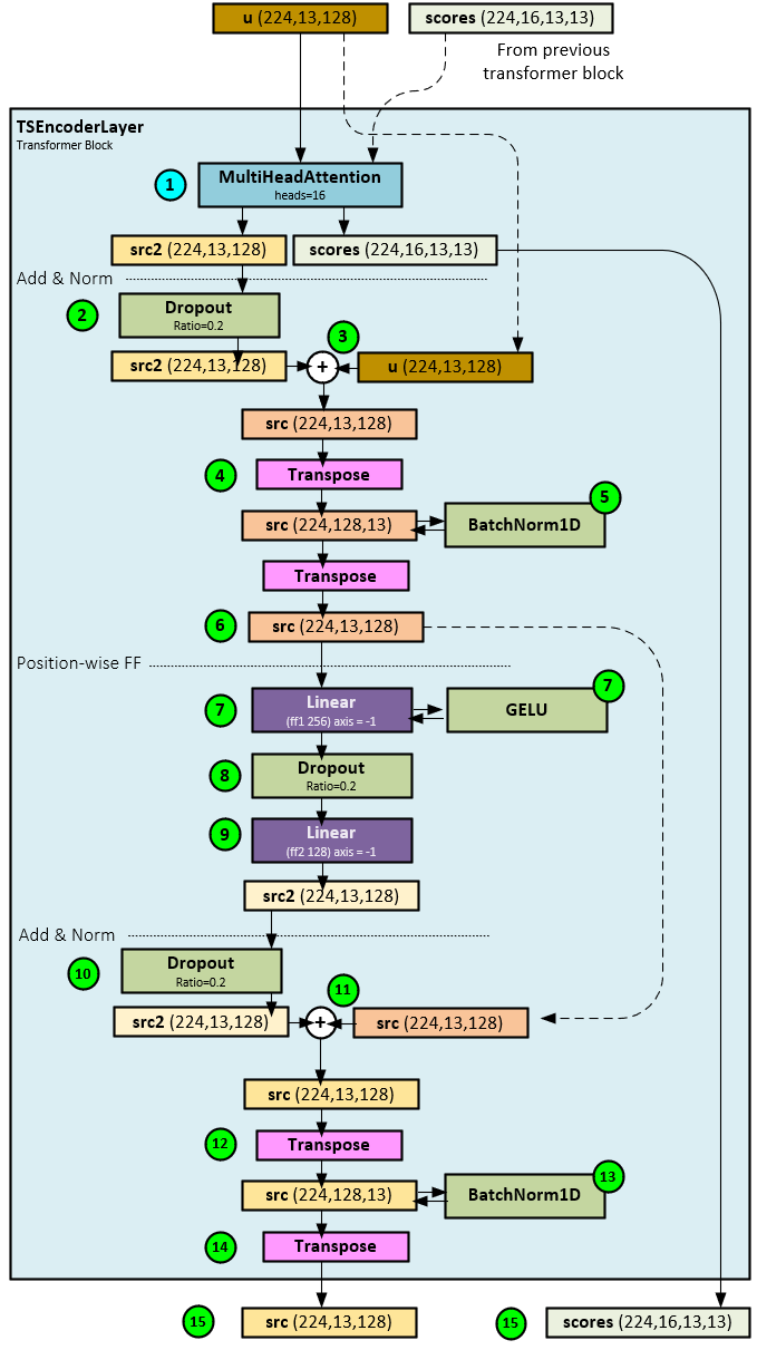
The following steps occur when processing the TSTEncoderLayer.
Attention
- First the u and previous layer scores tensors (if exists) are sent to the MultiHeadAttention layer with 16 heads for attention processing which produces the src2 and scores
Add & Norm
- The src2 tensor is passed through a Dropout layer with a dropout ratio of 0.2.
- Next, the original u tensor is added to the src2 tensor to produce a new src
- The new src tensor is transposed to the shape Batch * Channel x Transformer Data x Patch, …
- … and normalized with a BatchNorm1D
- The src tensor is then transposed back to the shape Batch * Channel x Patch x Transformer Data. Note steps 4-6 could be replaced with a LayerNorm layer but according to the paper, a BatchNorm1D may have better results. [1] (page 5) and [6].
Position-wise FF
- The src tensor is passed through a Linear layer that projects the src to a larger Transformer Data size. The result is run through a GELU activation layer.
- The projected src tensor is run through a Dropout layer with ratio = 0.2.
- A secondary Linear layer projects the src tensor back to its original size to produce a new src2
Add & Norm
- The src2 tensor is run through a Dropout layer with ratio = 0.2.
- Next, the src2 tensor is added to the original src tensor produced in Step #6 above.
- The new src tensor values are transposed to a new shape Batch * Channel x Transformer Data x Patch.
- The transposed src tensor is normalized with a BatchNorm1D layer, …
- … and transposed back to its original shape Batch * Channel x Patch x Transformer Data. Note, as noted in Step #6 above, steps 12-14 could be replaced with a LayerNorm layer but according to the paper, a BatchNorm1D may have better results. [1] (page 5) and [6].
- The final src and attention scores tensors are returned.
MultiHeadAttention Layer
The MultiHeadAttention layer performs a standard q, k, v self-attention on the u tensor input.
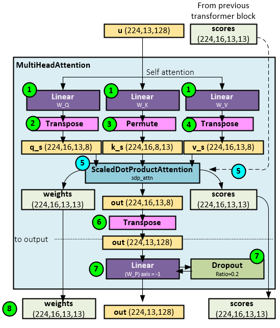
The following steps occur when running the MultiHeadAttention Layer.
- For self-attention, the u tensor is sent to each of the three W_Q, W_K and W_V Linear layers to produce the q, k and v values.
- The output of the W_Q Linear layer is reshaped and transposed to the shape Batch * Channel x Head x Patch x Transformer Data Piece (d_k) which becomes the q_s.
- The output of the W_K Linear layer is reshaped and permuted to the shape Batch * Channel x Transformer Data Piece (d_k) x Patch which becomes the k_s. Note the ordering of q_s and k_s is important when used in the scaled dot product attention discussed later.
- The output of the W_V Linear layer is reshaped and transposed to the shape Batch * Channel x Head x Patch x Transformer Data Piece (d_v) which becomes the v_s.
- All three tensors q_s, k_s, v_s and scores tensor (if exists) are sent to the ScaledDotProductAttention layer to produce the out, attention scores and attention weights
- The out tensor is transposed and reshaped to the shape Batch * Channel x Patch x Transformer Data.
- The reshaped out tensor is sent to Linear and Dropout layers in sequence to produce the final out
- The out, attention weights and attention scores tensors are returned.
Scaled Dot Product Attention Layer
The ScaledDotProductAttention Layer performs the actual attention calculations.
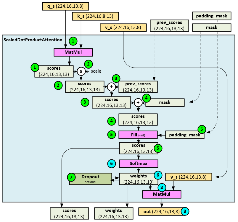
The following steps occur when calculating the attention in the ScaledDotProductAttention layer.
- First a MatMul of the q_s and k_s tensors produce the initial attention scores Note the transpose and permute used in the previous MultiHeadAttention layer discussion.
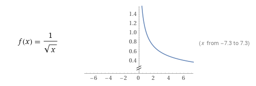
- Next, the attention scores tensor is scaled using the function f(x) shown below (image from Wolfram Alpha) where x = head dimension = model dimension / number of heads.
- If any previous attention scores exist from the previous TSEncoder Layer, they are added to the current attention scores
- If a mask exists, the values of the attention scores tensor are either set to -inf on the masked values when a Boolean mask is used, or the mask is directly added to the attention scores
- If a padding mask exists, the values of the attention scores tensor are set to -inf on the masked values.
- The final attention scores tensor is sent through a Softmax layer to produce the attention weights.
- Optionally, the attention weights tensor is sent through a Dropout layer (the default is to skip this step).
- The final attended out tensor and attention scores and weights tensors are returned.
Summary
We really like the PatchTST model for it reuses much of the transformer logic used in language model processing and does so in a very effective and efficient way by applying this architecture to predict patches, or small segments, pulled from each time-series stream to learn the time-series predictions. According to the paper, the PatchTST outperforms numerous other time-series models (DLinear, FEDformer, Autoformer, Informer, Pyraformer and LogTrans) by out predicting each on Weather, Traffic and Electricity datasets. [1] (pages 6-7) And, according to [7], the PatchTST outperforms the Temporal Fusion Transformer (TFT) as well.
Happy Deep Learning with the PatchTST model!
[1] A Time Series is Worth 64 Words: Long-term Forecasting with Transformers, by Yuqi Nie, Nam H. Nguyen, Phanwadee Sinthong, and Jayant Kalagnanam, 2022, arXiv:2211.14730
[2] How to understand “prediction” and “label” in classification?, by freak11, 2018, Stack Overflow
[3] GitHub: yuqinie98/PatchTST, by yuqinie98, 2023, arXiv:2303.06053
[4] Reversible Instance Normalization for Accurate Time-Series Forecasting against Distribution Shift, by Taesung Kim, Jinhee Kim, Yunwon Tae, Cheonbok Park, Jang-Ho Choi, and Jaegul Choo, 2022, GitHub
[5] RevIN (ICLR 2022) – Official PyTorch Implementation, by ts-kim, 2022, GitHub
[6] A Transformer-based Framework for Multivariate Time Series Representation Learning, by George Zerveas, Srideepika Jayaraman, Dhaval Patel, Anuradha Bhamidipaty, and Carsten Eickhoff, 2020, arXiv:2010:02803
[7] TSMixer: An All-MLP Architecture for Time Series Forecasting, by Si-An Chen, Chun-Liang Li, Nate Yoder, Sercan O. Arik, and Tomas Pfister, 2023, arXiv:2303.06053