

Change Point Detection (CPD) is an important field of time-series analysis that provides methods of detecting changes in mean, variance, and distribution structure within time-series data.
It has many applications in different fields, such as:
- Medicine: Change point detection can help monitor the health condition of patients, detect anomalies in vital signs, diagnose diseases, and evaluate the effects of treatments [1] [2].
- Aerospace: Change point detection can help detect faults in aircraft systems, identify abnormal events, and improve safety and reliability [1] [3].
- Finance: Change point detection can help analyze the trends and volatility of financial markets, detect frauds and anomalies, and optimize trading strategies [1] [3].
- Business: Change point detection can help monitor the performance and quality of products and services, detect customer preferences and behavior changes, and optimize marketing and pricing strategies [1] [3] [4].
- Meteorology: Change point detection can help study the patterns and variations of climate and weather, detect extreme events and natural disasters, and assess the impacts of human activities [1] [3].
- Entertainment: Change point detection can help analyze the popularity and ratings of movies, TV shows, music, and games, detect changes in audience preferences and feedback, and optimize content creation and recommendation [1] [3].
These are just some examples of the fields that use change point detection. There are many more fields that can benefit from this technique, such as biology, sociology, linguistics, and psychology. Change point detection is a powerful and versatile tool that can help us understand and explore the dynamics of complex systems [1]. (Portions generated with ChatGPT [5])
In this post we explore the neural network version of the Contrastive online change point detection (Algorithm II.1) as described in the article “A Contrastive Approach to Online Change Point Detection” by Goldman, et. al. Also see the original PyTorch source code for the article on GitHub here. As a base-line algorithm, we use the Cumulative Sum algorithm.
Cumulative Sum Change Point Algorithm
According to Wikipedia, the cumulative sum algorithm is a “sequential analysis technique developed by E.S. Page of the University of Cambridge” and is useful in change detection within a time-series of values. [1]
The implementation of the algorithm uses two loops where the outer loop traverses the input data from n = 0 to N-1, where N = the length of the data and the inner loop traverses a subset of the data from k = 0 to n-1. The inner loop produces prospective t-values that are calculated as the absolute difference between the mean of values before k and the mean of values after k up to n. On the completion of the inner loop, the maximum of prospective t-values produces the t-value for that value of n.
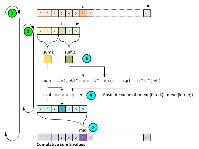
The following steps occur in the Cumulative Sum algorithm.
- The outer loop traverses each item of the input data where n = 0 to N-1.
- An inner loop traverses from k = 0 to n-1.
- On each step of the inner loop the values up to k and the values from k to n are summed to create sum1 and sum2 respectively.
- The two sums are used to create the mean up to k and the mean after k whose difference is used to calculate the prospective t-value candidate -which is placed in a temporary vector that is filled out by the inner loop.
- Upon completion of the inner loop, the maximum value of the temporary vector of prospective t-values becomes the t-value for that value of n in the S values vector.
As will be demonstrated layer, this simple algorithm is fast and accurate when detecting medium to large shifts in stationary data but struggles to detect small shifts and changes in variance.
See ChangePointDetectorCumulativeSUM.ComputeSvalues.cs for implementation details.
Contrastive NN Change Point Detection
According to the authors of “A Contrastive Approach to Online Change Point Detection”, the contrastive approach “expands an idea of maximizing a discrepancy between points from pre-change to post-change distributions.” [6] The algorithm highlighted in the article called Algorithm II.1 is as follows.
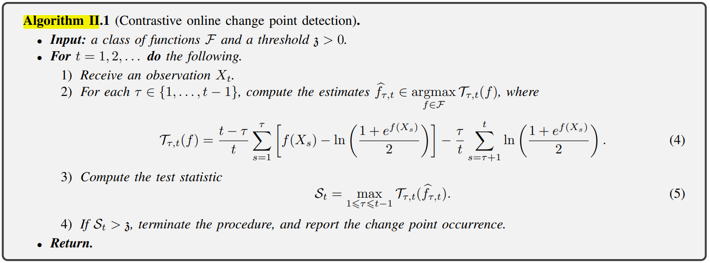
Algorithm II.1 is presented in two flavors, one that uses the Algorithm II.1 with polynomials of degree p and a second that uses the Algorithm II.1 with a fully connected feed-forward neural network.
We will be describing the second, neural network-based flavor as that is what is implemented in MyCaffe by the ChangePointDetectorContrastiveNN class.
How Contrastive NN Change Point Detection Works
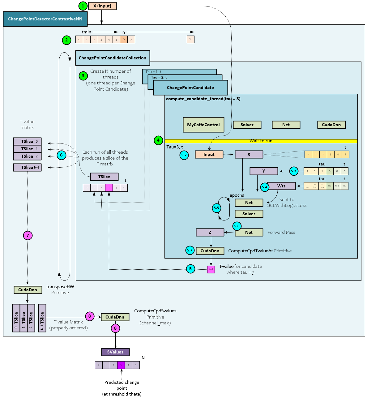
The MyCaffe ChangePointDetectorContrastiveNN class manages an internal set of ChangePointCandidate objects that each manage their own individual thread that trains their own internal neural network. ChangePointCandidates are independent of one another allowing each to run in parallel. See [7] for the original PyTorch version. Each ChangePointCandidate is assigned to a value of tau to process thereby producing the t-value at their assigned slot in the input data.
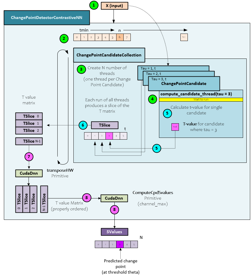
When calculating the S values, the following steps take place within the ChangePointDetectorContrastiveNN. S values are used to determine the change point location within the input X values.
- First the X input values are sent to the ChangePointDetectorContrastiveNN object for processing.
- The ChangePointDetectorContrastiveNN class processes each element n within the input X data in a main processing loop.
- At each iteration, a collection of ChangePointCandidate objects processes steps from 0 to the current n where a single ChangePointCandidate instance is assigned to each step. At the completion of the main loop the collection of ChangePointCandidates will have produced a matrix of prospective t-values.
- Each ChangePointCandidate is assigned to a different step and process their respective steps on separate, independent threads. All threads are synchronized to run at the same time when processing a slice of the T value matrix.
- On a given cycle, the internal thread of each ChangePointCandidate calculates the t-value at the specific Tau,T location (discussed in more detail later).
- The prospective t-value calculated is placed in the assigned location of the current TSlice being processed based on the Tau value.
- Once the T-value matrix processing completes, the MyCaffe low-level primitives are used to transpose the matrix.
- And the transposed T-value matrix is sent to the MyCaffe low-level primitive ComputeSvalues to compute the cpd S-value vector. This low-level primitive essentially performs a channel_max on the matrix to produce the final S value vector. Depending on the threshold used, the location that first breaches the threshold is the calculated change point location for the input data.
Change Point Candidate Processing
Each ChangePointCandidate object is responsible for computing the t-value at the candidates assigned Tau value run at a specific iteration t to fill out a slice within the T value matrix. The ChangePointCandidate uses a special compute_candidate thread to calculate the t-value.
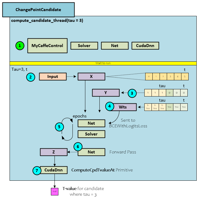
The following steps occur within the ChagePointCandidate thread to calculate the t-value candidate for a specific Tau value at iteration t in the data.
- During initialization an instance of MyCaffe is created for each thread. Once created, the internal Solver, Net and CudaDnn objects are accessed. After initialization, the thread waits for the run event to fire – which will occur when a new TSlice processing starts.
- When the run event fires, each thread starts processing their assigned Tau value within the Input (X) data. During this first step the external Input is copied to a local X blob which contains 0..t-1 items.
- Next, the Y virtual labels are created where all values up to tau are set to 1 and all other values are set to zero.
- The Wts blob is initialized to contain T-tau in the values up to Tau and all other values are set to Tau.
- An internal Neural Network is trained with these inputs for nEpoch number of iterations. Typically, the number of epochs ranges from 10 to 100 where 10 epochs are less accurate but quicker. We have found a range between 20 and 50 epochs to provide a good balance between accuracy and speed.
- Once training completes, a forward pass is run on the Net to produce the output Z predictions.
- The Z predictions are passed to the ComputeCpdTvalueAt MyCaffe primitive which calculates the candidate t-value using the Algorithm II.1 noted above.
The full Contrastive NN Change Point Detection architecture is shown below.
Neural Network Architecture
A very simple, fully connected, neural network is used in step #5 above with the following architecture created by the build_model method within the ChangePointCandidate object.
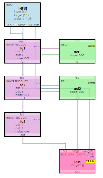
Inputs are passed to the input, target (Y), and weights blobs, and the loss is calculated via the BCEWithLogitsLoss layer. An Adam optimizer is used with a learning rate of 1e-1 and a fixed learning rate policy.
Change Point Detection Results
Our initial test results use simulated data created with an initial noise (sigma) level that has a data shift applied at the true change point. In some scenarios the noise is altered at the change point higher in some scenarios and lower in others.
A Box-Muller transform [8] is used to create a random value from a normal distribution see Randn function for more details.
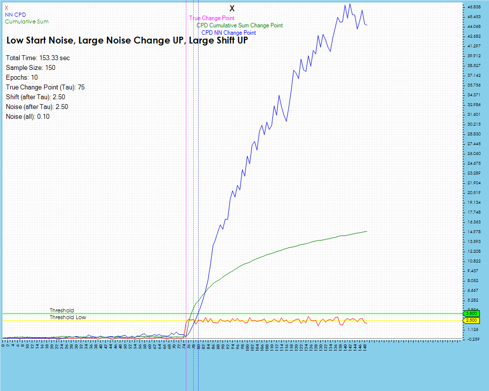
When detecting the change point in a data stream that has low noise and a relatively large data shift, the Cumulative Sum algorithm detects the change point very well, with little delay and does so very quickly. The Contrastive NN method has a very close, low lag result as well, but at the cost of a higher compute time.
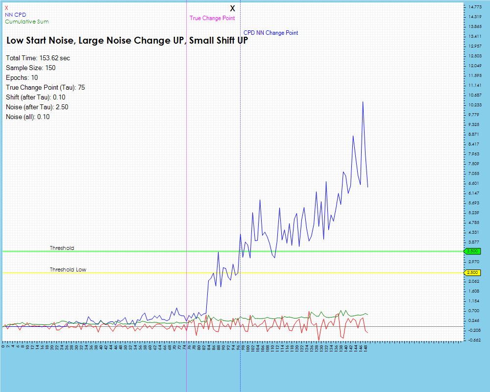
When running the same two methods on a data set containing a very small data shift at the change point, we see the Cumulative Sum algorithm does not even pick up the change whereas the Contrastive NN method does do so but with a longer lag than was observed with the larger data shift shown previously.
Impact of Epochs on Results
The number of epochs impact the amount of training run on each individual neural network, described above in Step #5 of the Change Point Candidate Processing. Longer training appears to have less impact on larger shifts in the data for the lag remains relatively the same.
The lag does decrease slightly when training with 50 and 100 epochs but only by one step. However, the lag decrease is much higher when processing data with smaller data shifts as shown below where the lag decreased by 38%.
However, this improvement comes at the cost of increased processing time.
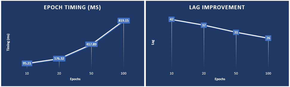
As the lag decreased by 38% the timing increased in sync with the number of epochs run from 95 milliseconds to run 10 epochs up to 819 milliseconds to run 100 epochs. These tests were run on a single NVIDIA RTX A6000 GPU.
Summary
In this post, we have discussed how the Cumulative Sum algorithm and Contrastive NN methods for change point detection work and have demonstrated how they differ when detecting change points.
Happy deep learning with Change Point Detection!
[1] Change detection, by Wikipedia
[2] Change Point Detection for Compositional Multivariate Data, by Prabuchandran K.J., Nitin Singh, Pankaj Dayama, and Vinayaka Pandit, 2019, arXiv:1901.04935
[3] A Review of Changepoint Detection Models, by Yixiao Li, Gloria Lin, Thomas Lau, and Ruochen Zeng, 2019, arXiv:1908.07136
[4] A Review of Changepoint Detection Models, by Christof Schroth, Dr. Julien Siebert and Janek Grob, 2021, Fraunhofer
[5] Chat-GPT, by OpenAI, 2023
[6] A Contrastive Approach to Online Change Point Detection, by Artur Goldman, Nikita Puchkin, Valeriia Shcherbakova, and Uliana Vinogradova, 2022, arXiv:2206.10143
[7] GitHub:nupuchkin/contrastive_change_point_detection, by npuchkin, 2022, GitHub
[8] Box-Muller transform, by Wikipedia