

As discussed in our previous post, Change Point Detection (CPD) is an important part of time-series analysis used in numerous fields such as Medicine, Aerospace, Finance, Business, Metrology and Entertainment.
In this post, we expand our analysis of an adaptive, online algorithm for Change Point Detection based on the paper “Memory-free Online Change-point Detection: A Novel Neural Network Approach” by Atashgahi et. al. which describes the Adaptive LSTM-Autoencoder Change Point Detection (ALACPD) algorithm [1]. The original TensorFlow implementation of ALACPD, described in this post is available on GitHub at [2].
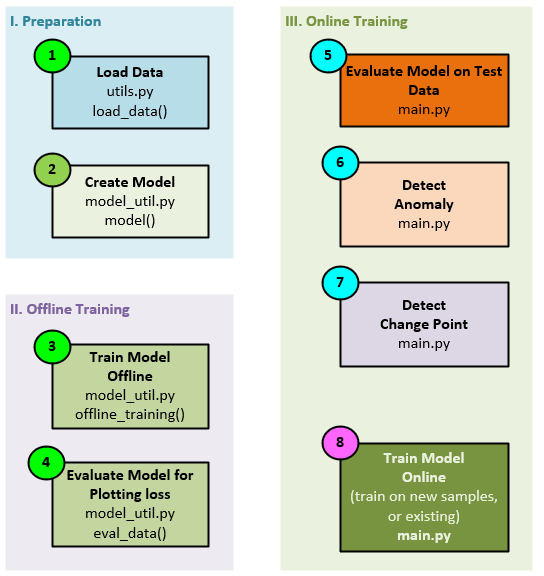
There are three main phases to the ALACPD algorithm: 1. Preparation, 2. Offline Training, and 3. Online Training.
Change Point Detection Algorithm
The basic algorithm of the ALACPD to detect change points in an unsupervised manner is uses an ensemble of 3 or more identical models (all with different, randomly initialized weights) that are all run on the current input data. Upon detecting a consensus of models calculating losses higher than a given threshold, it is determined that an anomaly has been found, but not yet a change point. Upon detecting an anomaly consensus 3 more consecutive times, the anomaly is determined to be a change point.
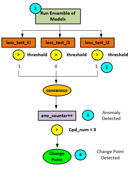
The following steps occur when detecting change points.
- The ensemble of 3 or more models is run on the same data (the randomly initialized weights will be slightly different after off-line training) to produce the corresponding 3 or more loss values.
- A count of loss values exceeding a pre-specified threshold is made.
- If a consensus of counts exceeds the threshold an anomaly has been detected and the anomaly counter is increased. If no consensus is reached, the anomaly counter is reset to zero.
- Once the anomaly counter exceeds the change point detection number a change point has been detected. For example, if the change point detection number = 3, a change point is detected after four consecutive anomalies have been detected.
ALACPD Results
For the following results, the original APACPD model [2] was run on the SPY ETF adjusted close prices over the past 5 years, from 2019 to December 2023. This period covers both the COVID crash and large rally that followed.
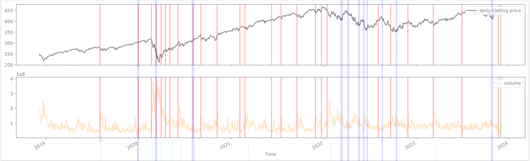
After running the ALACPD algorithm a number of change points (red lines) were detected – we manually added blue bar annotations where change points were either missed or detected without data support.
From a visual inspection, we can see that the model does detect change points well but has a few missing gaps. For example, it is unclear why the model did not detect any change points during the 2022 downturn even though there were many price and volume variations during that time period that would appear to be clear change points.
Now we will discuss how each of the three phases of this adaptive change point detection model work.
Phase 1 – Preparation
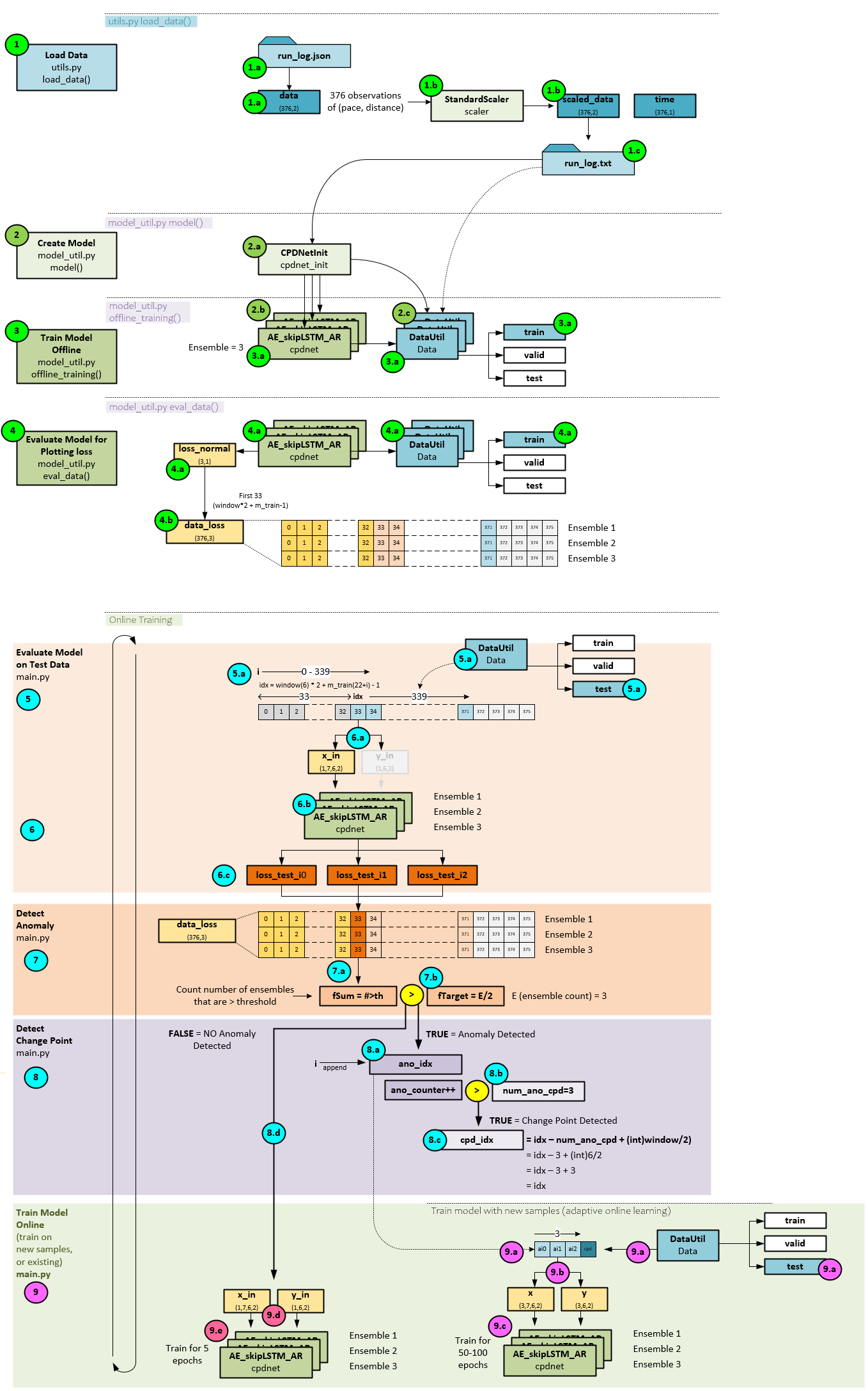
During the preparation phase, the data is preprocessed, loaded, and the models are created. Data preprocessing involves loading the data from a Json file, scaling it with the StandardScaler, then saving the scaled data to a text file.
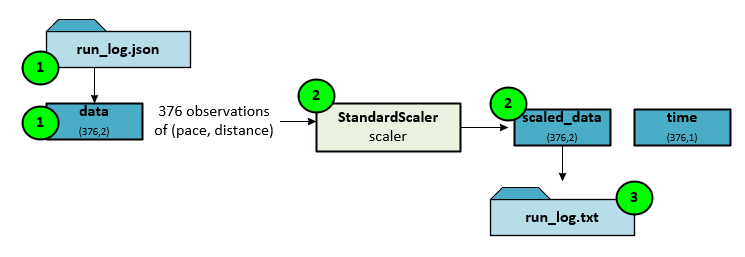
The following steps occur during data preprocessing.
- First the Json file is loaded into the data numpy array with a shape of (observations, dimensions).
- The data numpy array is then scaled using the StandardScaler which centers and scales the data to a unit variance.
- The scaled data is then saved to a text file later load during the training phases.
The data pre-processing is performed by the load_data function in the utils.py file.
Loading The Data
During the preparation phase, the data is loaded into a DataUtil object that manages the train, test, and valid datasets, all originating from the text file of data previously discussed.
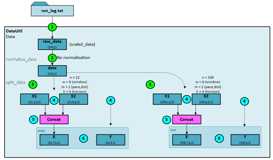
During the data loading process, the following steps occur.
- The data text file is loaded into the raw_data numpy array with a dimension of (observations, dimension).
- Since the data was previously normalized during the data preparation step, no new normalization occurs and the raw_data is copied to the data numpy
- Next, the split_data method creates the train and test datasets.
- When creating each dataset, the data is organized into X1 and X2 numpy arrays (described later). The Y targets are created as well.
- The X1 and X2 numpy arrays are concatenated together to create the X.
- Both the training and testing data sets are loaded with their own, separate X and Y
Data Organization
The run_log.txt dataset contains pace and distance data for a long-distance runner and has 376 observations. The first thirty-seven (0.1 * 376) of the observations make up the training dataset used for offline training. A data window = 6 and horizon = 4 are used to build the dataset with the starting index for the build set at window * 2 + horizon – 1, which equals 15. Of the 37 observations, with offsetting, there are 22 items in the training set.
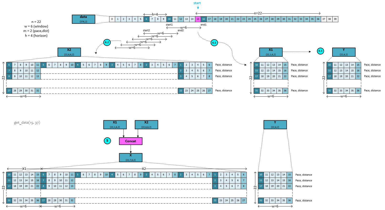
When loading the data into the DataUtil object, the following steps occur in the get_data function within the cpdnet_datautil.py file.
4.1) The X1 numpy array is created with shape (22, 1, 6, 2) where there are a total of 22 observations used in the training set, 6 items make up the data window and 2 dimensions make up the pace and distance dimensions. Six windows of data are loaded into the X1 numpy where each window contains data starting in steps progressing forward by one step. So, the first window contains items 10 to 15, the next 11 to 16, the next 12 to 17 and so on. 22 such windows are stacked to make up the X1 data.
4.2) The X2 numpy array is created with shape (22, 6, 6, 2) where there are a total of 22 observations used in the training set, 6 items make up a data window, and 2 dimensions make up the pace and distance dimensions. Six windows of data are loaded into each row of the X2 numpy where each window precedes the other by one step back in the data. For the first row, the window from index 6 to 11 is then followed by the window from 5 to 10, followed by 4 to 9 and so on. Since multivariate data is processed, each item contains both the value for pace and distance. The next row of X2 contains a similar organization but starting 1 step forward in the data, which essentially creates a matrix of values that naturally highlight large changes that are repeated across the matrix.
4.3) The Y value is merely a copy of the X1 data.
Phase 2 – Offline Training
The offline training phase is used to ‘warm-up’ the model by pre-training on the small training set of data. Once trained, the model is evaluated to create the initial loss_normal values.
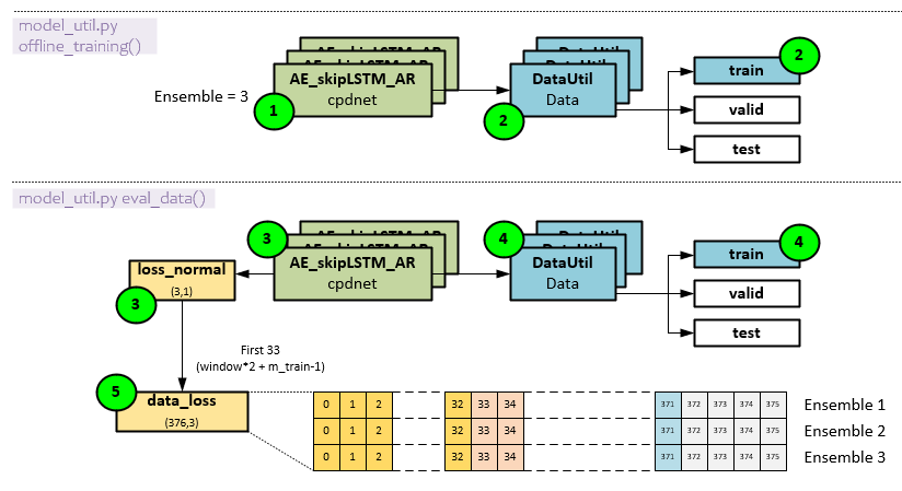
The following steps occur during offline training.
- First the ensemble of models is trained.
- During training, the DataUtil feeds batches of data from the training set using the data ordering previously discussed.
- Next, the model ensemble is evaluated to produce a new set of loss_normal
- The training data set is used for the evaluation.
- The loss_normal values are added to the off-line training section of the input data stream. The data_loss values are used for model analysis and plotting.
Phase 3 – Online Training
The online training consists of detecting anomalies, determining if those anomalies are actual change points and then adaptively training the model on new data to better fit the dynamics of the data stream moving forward.
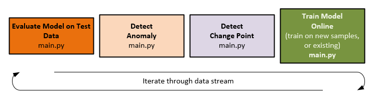
Online training cycles through each item in the test data stream one item at a time until the end of the data stream or until new data arrives in a real-time scenario.
Evaluate Mode on Test Data
The model ensemble evaluates the data at the current data idx within the training dataset to produce the loss values for each model within the ensemble.
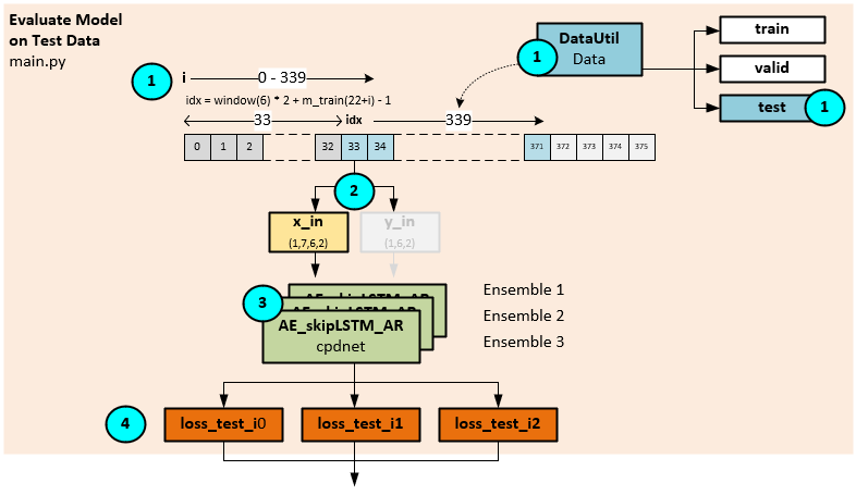
The following steps occur during the model evaluation.
- The DataUtil builds the data packet for the current index in the training dataset (as described in Data Organization above).
- The data packet makes up the x_in and y_in values, yet only the x_in is used during the evaluation step.
- The ensemble of models is run through a forward pass to evaluate the data…
- …and produces the ensemble of corresponding loss values loss_test_i0, loss_test_i1, and loss_test_i1.
Anomaly Detection
During anomaly detection, a count of all loss values exceeding a pre-specified threshold is taken. If a consensus of models in the ensemble is above the threshold an anomaly is detected.
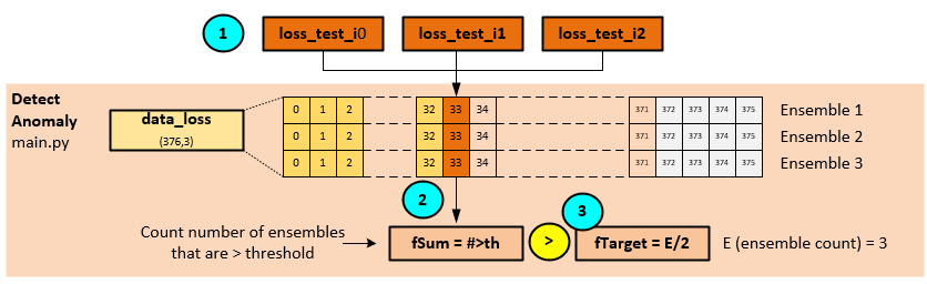
The following steps occur when detecting an anomaly.
- Using the loss values output from the model ensemble evaluation…
- … a count of loss values exceeding an external threshold is taken.
- If a consensus of losses (e.g., 2 of 3) exceed the threshold, an anomaly is detected.
Change Point Detection
On detecting each anomaly, an anomaly counter is increased, and once a pre specified number of consecutive anomalies is found, a change point is detected.
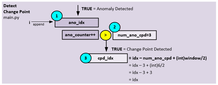
The following steps occur during change point detection.
- On detecting an anomaly, the current index in the training data set is appended to the ano_idx collection (later used during on-line training). Next, the anomaly counter is increased.
- Once the anomaly counter of consecutive anomalies exceeds a pre specified anomaly counter threshold (e.g., num_ano_cpd = 3) …
- … it is determined that a change point has been detected at the index.
Online Training (Adaptive Learning)
During on-line training, there are two methods of training, one method that occurs when no anomaly is detected, and the other that occurs when a change point is detected.
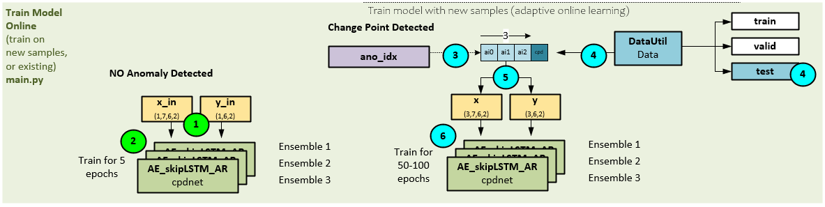
The following steps occur in an on-line training cycle where no anomalies are found.
- In the case where no anomaly is detected, the same data originally evaluated during the Evaluate Model on Test Data step described above is used for training.
- A short 5 epoch training cycle is run on the original x_in, y_in
The following steps occur in an on-line training cycle where a change point is found.
- During the detection of change points, the indexes of each anomaly are saved in the ano_idx array. The data values at these indices are now used during training.
- The test data from the DataUtil is used to build the input data by…
- …extracting the data from the test data at the ano_idx indexes to create the x and y.
- The ensemble of models is trained on the x and y arrays for 5o to 100 epochs.
ALACPD Full Process
For the full ALACPD Change Point Detection process with adaptive learning, click on the image below.
Model Details
Now that you have a better understanding of how the change detection algorithm works, what about the model itself? The ALACPD algorithm uses a custom LSTM layer called the Skip LSTM with Autoregression, or AE_skipLSTM_AR for short. The model ensemble comprises 3 or more of the same AE_skipLSTM_AR models.
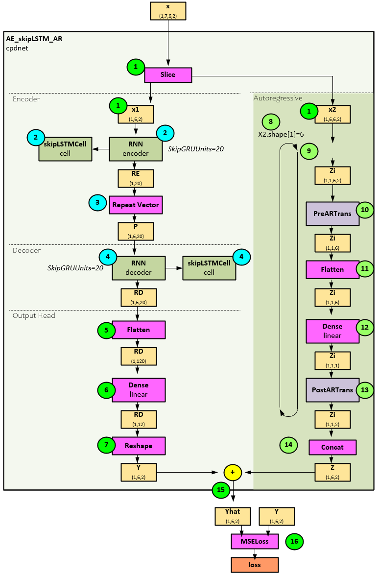
When processing the X input to produce the Yhat predictions, the model takes the following steps.
- First the X (1,7,6,2) input is sliced into the X1 (1,1,6,2) and X2 (1,6,6,2) tensors.
- The X1 tensor is fed into an RNN encoder layer that uses the specialized skipLSTMCell for the encoder processing.
- The RE output is repeated six times to create the P tensor.
- The P tensor is then fed into the RNN decoder layer that uses the specialized skipLSTMCell as well to produce the RD tensor.
- A Flatten layer changes the RD (1,6,20) to RD (1,120) by flattening the last two axes.
- The flattened RD is fed into a Dense linear layer to produce the RD (1,12) output.
- A Reshape layer splits the last two axes into the Y (1,6,2) tensor.
- Next, the auto regressive steps start processing the X2 tensor by looping through each of the 6 items in the X2 (1,6,6,2) shape[1]. The following steps occur at each iteration.
- First the X2 is split into the tensor at that iteration to create the Zi (1,1,6,2) tensor.
- A PreARTrans is used to reformat the Zi for the autoregression steps.
- The Zi tensor is then flattened to the shape (1,1,6) …
- … and run through a Dense linear layer to produce the Zi (1,1,1) output.
- A PostARTrans is run to reformat the data back producing the Zi (1,1,2) tensor. The loop continues back at step 9 until each of the 6 items in the tensor are processed.
- All Zi tensors are concatenated into the Z (1,6,2) output.
- The Z tensor is added to the Y from step #7 above to produce the Yhat (1,6,2) output.
- An MSELoss layer is run to calculate the loss between the Yhat and Y tensors to produce the final output loss value.
SkipLSTMCell Layer
Both the RNN encoder and RNN decoder layers use the skipLSTMCell layer for processing each step within the respective recurrent neural networks.
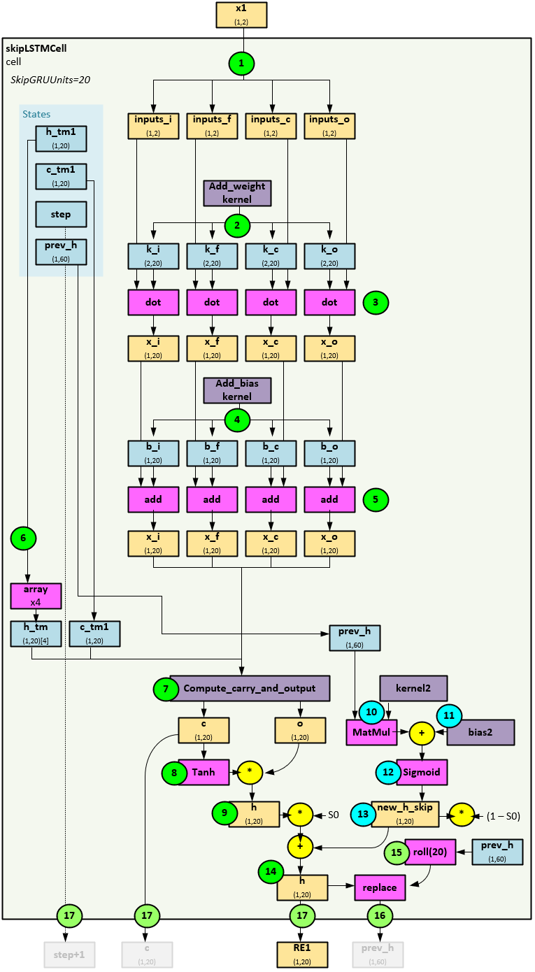
When processing the x1 input at each step of the RNN, the skipLSTMCell layer takes the following steps to produce the RE1 output for the input item.
- First the X1 input is copied into the inputs_i, inputs_f, inputs_c and inputs_o tensors all with shape (1,2).
- Next, the Add_weight kernel is used to create the k_i, k_f, k_c, and k_o weights each of shape (2,20).
- The inputs and k weights are each run through a dot operation to produce the x_i, x_f, x_c and x_o tensors of shape (1,20).
- Next the Add_bias kernel is used to create the b_i, b_f, b_c, and b_o bias values each of shape (1,20).
- The bias values are added to the previous x values to produce the x_i, x_f, x_c and x_o tensors of shape (1,20).
- Next, the h_tm1 weights are duplicated into a 4-element array h_tm.
- The copute_carry_and_output function is run to produce the c and o tensors (more on this later).
- The c tensor is run through a Tanh and multiplied by the o tensor…
- … and the result produces the h tensor (which will later be used to update the prev_h tensor).
- A MatMul is performed between the prev_h (1,60) tensor and the kernel2 weights and the results…
- …are added to the bias2 weights, whose results are…
- … run though a Sigmoid function to produce the new_h_skip (1,20) tensor.
- The new_h_skip tensor is multiplied by (1-S0) where S0 is a hyper parameter and added to the h (1,20) tensor multiplied by S0.
- This produces the new, updated h tensor (that is later returned as RE1).
- The prev_h tensor is updated by first rolling the tensor…
- … which allows for the old h values to be replaced with the new as the prev_h tensor of size (1,60) holds three sets of h (1,20) tensor values.
- The h tensor (1,20) is returned as the RE1. The step + 1, c and prev_h tensors are also returned, but not used.
compute_carry_and_output Function
The compute_carry_and_output function called previously in step #7, calculates the o and c gate values.
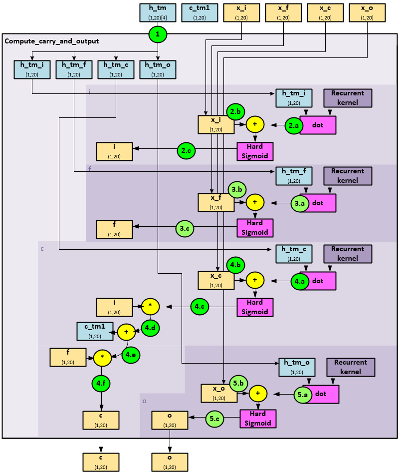
The following steps occur within the compute_carry_and_output function when calculating the o and c gates.
- First the array of h_tm (1,20)[4] values are separated into the h_tm_i, h_tm_f, h_tm_c, and h_tm_o tensors.
- Next, the i gate is processed.
- A dot is performed between the h_tm_i (1,20) weight and associated recurrent kernel weights.
- The result is added to the x_i (1,20) input tensor…
- … and run through a Hard Sigmoid to produce the i (1,20) gate tensor.
- Next, the f gate is processed.
- A dot is performed between the h_tm_f (1,20) weight and associated recurrent kernel weights.
- The result is added to the x_f (1,20) input tensor…
- … and run through a Hard Sigmoid to produce the f (1,20) gate tensor.
- Next, the c gate is processed.
- A dot is performed between the h_tm_f (1,20) weight and associated recurrent kernel weights.
- The result is added to the x_c (1,20) input tensor…
- … and run through a Hard Sigmoid whose result…
- … is multiplied by the i (1,20) gate tensor, and…
- … added to the c_tm1 weight tensor, then…
- … multiplied by the f (1,20) gate tensor to produce the c (1,20) gate tensor.
- And finally, the o (1,20) gate is processed.
- A dot is performed between the h_tm_o (1,20) weight and associated recurrent kernel weights.
- The result is added to the x_o (1,20) input tensor…
- … and run through a Hard Sigmoid to produce the o (1,20) gate tensor.
Both the c (1,20) and o (1,20) gate tensors are returned.
PreARTrans and PostARTrans
The PreARTrans run in step #10 is used to reformat the Zi data for autoregressive processing and the PostARTrans run in step #13 is used to reverse the formatting.
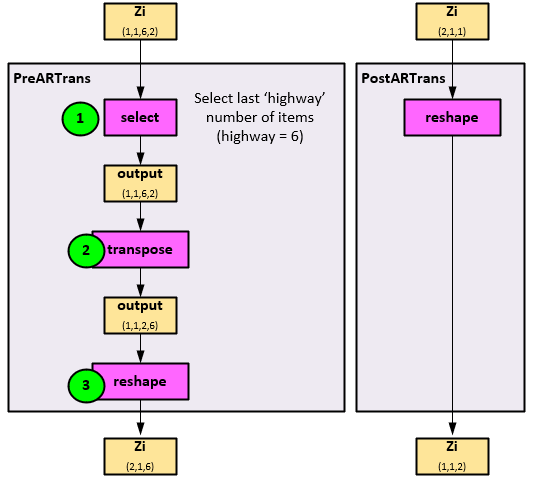
The following steps occur in the PreARTrans to alter the Zi (1,1,6,2) input.
- The last ‘highway’ number of items is selected from the Zi axis 2 where the highway is a hyperparameter. In this case the highway=6 and is the same size as the axis 2 shape, so no alteration occurs, and the output tensor is of shape (1,1,6,2).
- Next, the output tensor is transposed along the last two axes to produce a new output of shape (1,1,2,6).
- The output is then reshaped to produce the final Zi tensor of shape (2,1,6)
The PostARTrans reshapes the data back to its original sizing of Zi (1,1,2).
Summary
In this post we have discussed how the ALACPD algorithm works to detect change points in an unsupervised manner by detecting a consensus of increased loss values return from an ensemble of models that each use specialized LSTM layers.
We discuss the overall off-line and on-line processes used to adaptively learn new data patterns and have shown in depth how these models work. And we have shown the results of running this model on 5 years of SPY ETF daily data showing the power and challenges of adaptive learning non-stationary data.
Happy Deep Learning!
[1] Memory-free Online Change-point Detection: A Novel Neural Network Approach, by Zahra Atashgahi, Decebal Constantin Mocanu, Raymond Veldhuis, and Mykola Pechenizkiy, 2022, arXiv:2207.03932
[2] GitHub:zahraatashgahi/ALACPD, by zahraatashgahi, 2022, GitHub