Understanding TFT Momentum Rebalancing for High Sharpe Ratios

In this post we describe the Temporal Fusion Transformer based Momentum Rebalancing Transformer described in the paper, “Trading with the Momentum Transformer: An Intelligent and Interpretable Architecture” by Wood et. al. [1], published in 2022. The original code analyzed can be found on GitHub at [2].

Time-series momentum (TSMOM) strategies such as ‘buying the winners and selling the losers’ [3] have been around for over 20 years. In such strategies, the top performing assets are bought whereas the bottom performing assets are sold [4].

A recent approach for time-series momentum trading uses Deep Momentum Networks (DMN) to learn sizing of both trend and position “by directly optimizing on the Sharpe ratio of the signal. … [However] even DMNs have been underperforming in recent years, … [for they] struggle with long term patterns and responding to significant events…” [1]

The Momentum Transformer “is a subclass of DMN’s which incorporates [the] attention mechanisms” [1] of the Temporal Fusion Transformer (TFT) [5] model discussed in one of our previous posts. The Momentum Transformer uses the ‘fusing’ features of the Temporal Fusion Transformer to merge data with synthetic data. The data fusion is then fed through the model and to a new SharpeLoss layer that optimizes the model toward asset position sizes that maximizes the Sharpe ratio over time.

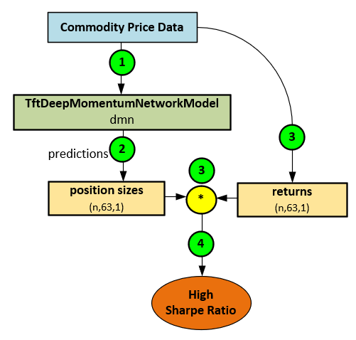
In general, the Momentum Transformer learns from Commodity Price Data (1) to make position size predictions (2) that when combined with known returns (3) produce a high Sharpe ratio (4).

Preliminary Results

For our preliminary results, we ran the TFT-SHORT model configuration which uses a total of 63 temporal steps and trained for a total of 300 epochs using the Adam optimizer. No change points are used in this configuration.

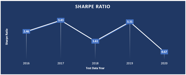
The following table shows the annual Sharpe ratio reached for the five years 2016-2020. Results for each year were produced after training for all years with data prior to the year in which the tests were conducted. For example, for the 2016 test results, training ran on years from 1990 to the end of 2015. For the 2017 test results, training ran in the years from 1990 to the end of 2016 and so on.

The results shown are for tests run with a sliding window of data, using the following hyper parameters.

Maximum Gradient = 1.0
Learning Rate = 0.01
Hidden Layer Size = 10
Dropout Ratio = 0.1
Batch Size = 256

All Sharpe ratios were reached when training on commodity data, using the original project code available on GitHub at [2].

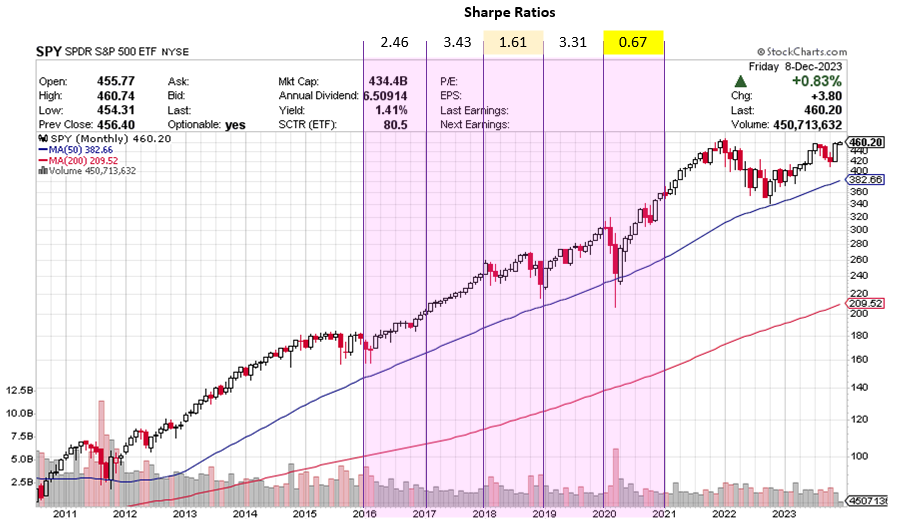
From the preliminary results, run on commodity data, the model looks very promising – however the model was adversely affected by the large COVID crash of 2020 where the worst Sharpe Ratio of 0.67 was observed.

Momentum Transformer Overall Process

A new TftDeepMomentumNetworkModel makes up the TFT + SharpeLoss model used to optimize the Sharpe ratio based on a rebalancing of assets over time. Rebalancing is performed on a selection of assets from 100 commodity futures (data available from Nasdaq Data Link). The rebalancing is run over 6 different time periods where the last year is used as the testing dataset with the previous years back to 1990 being used for the training dataset. Of the several model variants that are supported in the original implementation [2], this post focuses on the “TFT-SHORT” model that uses the TFT model only (without change points, used in other models) and a 63-step sequence.

The following steps make up the Momentum Transformer Processing.

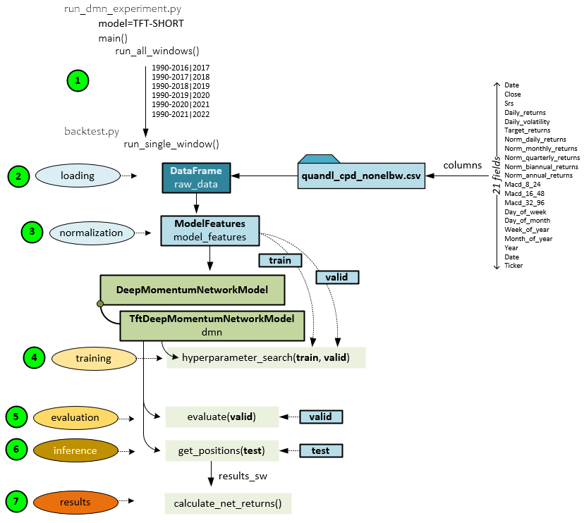
Datasets from 6 date range ‘windows’ are run through the model independently to produce a Sharpe ratio and overall performance rating for each. The run_all_windows function runs each of the date ranges by calling the run_single_window function to process a single window of data. For example, the date range 1990-2016 used for training and 2017 used for testing is processed by one call to the run_single_window
First all data from the data window is loaded from the csv file (previously created by running the create_features_quandl.py script). The csv file has the following columns of data: Date, Close, Srs, Daily returns, Daily volatility, Target returns, Normal daily returns, Normal monthly returns, Normal quarterly returns, Normal biannual returns, Macd(8,24), Macd(16,48), Macd(32,96), Day of week, Day of month, Week of year, Month of year, Year and Ticker.
The raw data is loaded into the ModelFeatures and normalized.
The TftDeepMomentumNetworkModel performs several tasks, the first of which is to find the optimal hyper parameters by training the model over and over on hyper parameters selected using a customization of the Keras RandomSearch This search is performed in the hyperparameter_search function.
The best trained model found in step #4 above, is then evaluated by running inference over the validation dataset (the last 10% of the training set). For example, in the first data window run, the testing dataset covers the last 10 % of the training data for years 1990-2016.
To predict the rebalancing results, the model is then run over the testing dataset which covers a full year of data. For example, in the first window of data trained from 1990 through 2016, the test dataset comprises the year of 2017. This inferencing occurs within the get_positions function and produces the results_sw comprising the results calculated over a sliding window of data.
The results_sw data is sent to the calc_net_returns function to calculate the final returns for the rebalancing occurring during year of data in the testing dataset.

Each of these steps are discussed in more detail in the following sections of this post.

Step 1 – Data Preparation

The data preparation stage involves converting the raw commodity data (downloaded from Nasdaq Data Link) into the quandl_cpd_nonelbw.csv data file. During this process, the target returns, and normalized inputs are created.

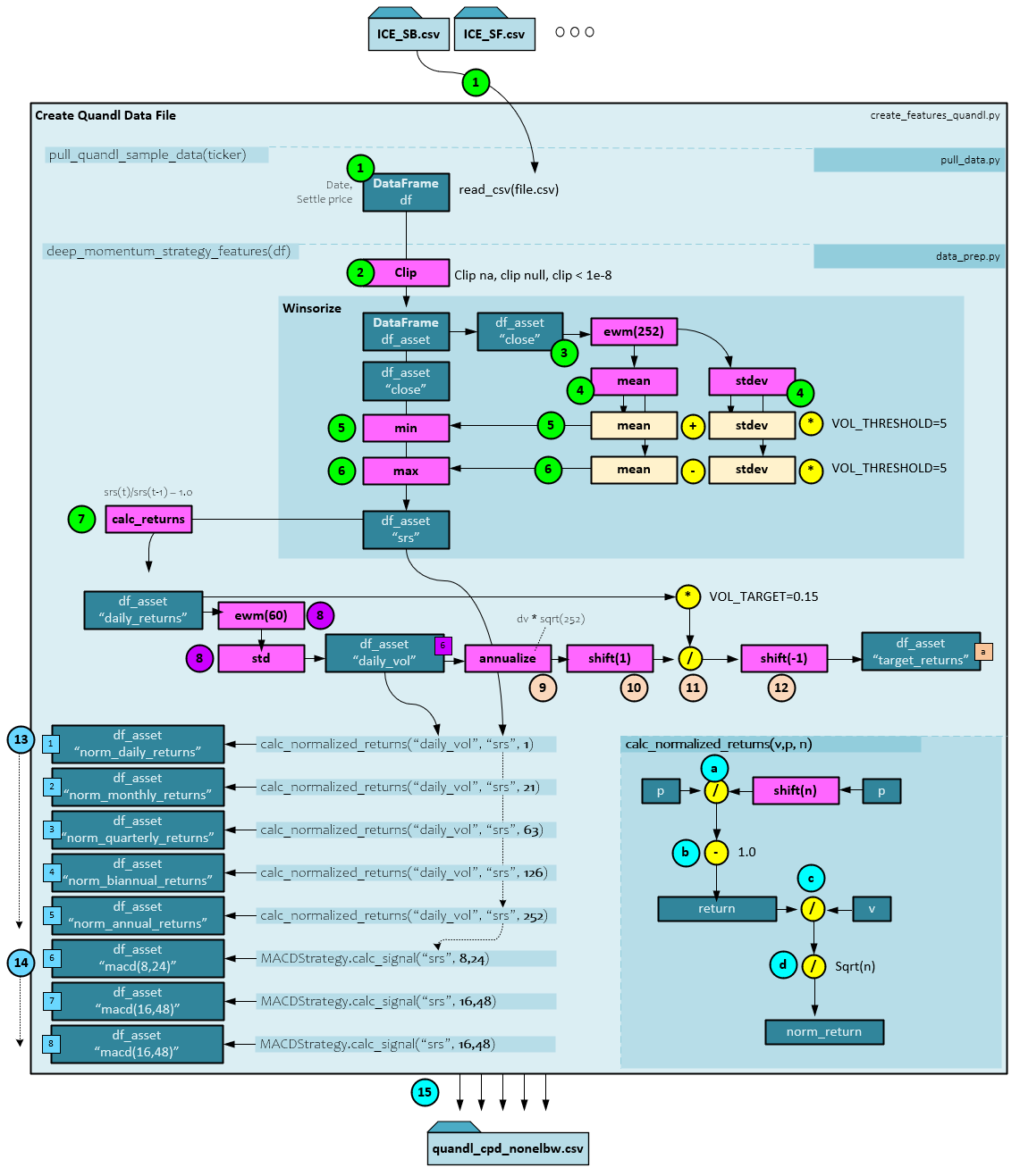
During the data preparation the following steps occur.

Each of the raw data files located within the data\quandl directory are loaded and processed using the steps below. All raw data files are downloaded using the py script. Each raw data file is named with the associated commodity symbol and contains a list of day date and settle prices for the commodity. The raw CSV data file is loaded into a DataFrame using the Pandas read_csv() function.
Next, the missing values, null values and values less than 1e-8 are clipped from the data to produce the df_asset DataFrame.
The ‘close’ price is extracted from the DataFrame and an ExponentialMovingWindow is created with the ewm function to exponentially weight with a halflife = 252 winsorize periods.
An ExponentialMovingWindow mean and standard deviation are taken of the ‘close‘ prices.
The ‘close’ is set to the minimum of the ewm mean + the ewm stdev * a VOL_THRESHOLD = 5.
The ‘close’ is then set to the maximum of the ewm mean – the ewm stdev * a VOL_THRESHOLD = 5. The results become the ‘srs’ value set in the df_asset DataFrame.
Next the daily_returns are calculated by the calc_returns function which uses the following function: ’daily_returns’ = srs(t) / srs(t-1) – 1.0. The daily_returns are set in the df_asset DataFrame.
Next the daily_vol values are calculated by running the daily_returns through an ewm function with span and min_periods set to VOL_LOOKBACK=60. A standard deviation is taken of the emw result to produce the daily_vol values which are set in the df_asset DataFrame.
The next four steps are taken to create the target_returns First the daily_vol values are annualized by multiplying by the square root of 252.
Next, a shift(1) is performed on the annualized daily_vol.
The shifted +1 annualized daily_vol is then divided by the daily_returns multiplied by the VOL_TARGET = 0.15 for 15%.
The result of step #11 is then shifted -1 to produce the final target_returns.
Next the normalized returns for the daily_returns are calculated for daily, monthly, quarterly, biannual, and annual periods. The following sub-steps are taken to normalize over each period.
1. First the input returns ‘p’ are divided by a shift of n periods back in time.
2. One (1.0) is then subtracted from the result of step #a above to produce the returns.
3. To normalize, the returns are divided by the daily volatility v…
4. … and then divided by the square root of n periods to produce the norm_returns.
A MACD is calculated with several different short and long periods to produce the three MACD input signals. See the MACD Calculation below for more details.
The ‘srs’, ‘daily_returns’, ‘daily_vol’, ‘target_returns’, all normalized returns, and all MACD values are saved to the csv file.

MACD Calculations

The MACD or ‘Moving Average Convergence/Divergence Oscillator’ is a popular signal used by many equity and commodity traders.

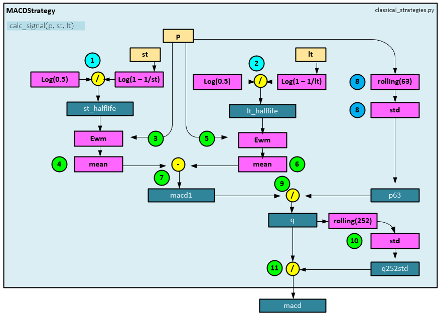
The inputs to the MACD include the value stream ‘p’ along with a short and long period such as 8 and 24. Calculating the MACD involves the following steps.

The st_halflife is calculated by dividing the log(0.5) by the log(1 – 1/st) where the ‘st’ is the short period (e.g., 8).
The lt_halflife is calculated by dividing the log(0.5) by the log(1 – 1/lt) where the ‘lt’ is the long period (e.g., 24).
An ExponentialMovingWindow is created by the ewm function with a halflife = st_halflife.
The ExponentialMovingWindow mean is taken of the stream ‘p‘ values.
An ExponentialMovingWindow is created by the ewm function with a halflife = lt_halflife.
The ExponentialMovingWindow mean is taken of the stream of ‘p‘ values.
The long-term result from step #6 above is subtracted from the short-term result from step #4 to produce the macd1 value.
A 63-period rolling standard deviation is taken of the value stream ‘p’ to produce the p63 value.
The macd1 is divided by the p63 rolling standard deviation to produce the ‘q’ value.
A 252-period rolling standard deviation is taken of the value stream ‘q’ to produce the q252std value.
The q value is then divided by the q252std value to produce the final macd value.

Moving ahead, the next steps start by using the quandl_cpd_nonelbw.csv file.

Step 2-3 – Data Loading and Preprocessing

Before the models are trained and evaluated, the raw data is loaded from the quandl_cpd_nonelbw.csv file and preprocessed. Data preprocessing involves normalization and separating the data into batches for training.

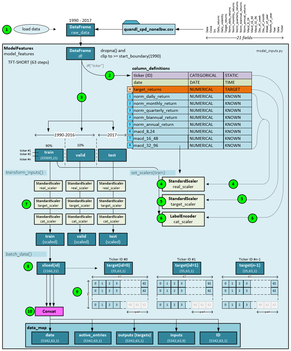
The following steps occur during data preprocessing.

First the data from the csv file falling within the data window (e.g., 1990-2017) is loaded into a Pandas DataFrame.
The DataFrame is passed to the ModelFeatures object which first removes missing data with dropna() and clips any data older than 1990. Column definitions are designated for the data consisting of 11 columns: ticker, date, target returns, norm daily return, norm monthly return, norm quarterly return, norm biannual return, norm annual return, macd(8,24), macd(16,48) and macd(32,96). Each column is assigned a stream class (e.g., CATEGORICAL, NUMERICAL, etc.) and value class (e.g., STATIC, TARGET, KNOWN, UNKNOWN). These classifications define the inputs to the Temporal Fusion Transformer.
Next, the DataFrame is split into the train, valid and test datasets where the test dataset includes the last year of data in the data window (e.g., 2017), and the train and valid include the data up to that last year (e.g., 1990-2016) where the valid contains the last 10% of the training data range and the remaining 90% is assigned to the train.
The train dataset is used to set the StandardScaler for the 8 numerical (real) data columns (norm daily return, norm monthly return, norm quarterly return, norm biannual return, norm annual return, macd(8,24), macd(16,48) and macd(32,96)).
The train dataset is also used to set a separate StandardScaler for the target numerical (real) data column.
And a LabelEncoder is set for the ticker column of the train.
Next, the transform_inputs() function transforms the inputs using the scaler objects set in steps 4-6 above. The StandardScaler centers the data and scales to a unit variance scale, whereas the LabelEncoder converts the text ticker names into numerical index values. The scaling process produces the scaled train, valid and test.
Next, the batch_data() function builds batch ready slices of the data organized into 63 steps each. To create the batch ready slices, the dataset processed (e.g., train, valid or test dataset) is cut into slices where each slice contains the data associated with a single ticker. For example, a single slice will contain all data for the ICE_SB symbol (Sugar Futures).
Each slice is then organized into non-overlapping sequences of 63 steps each. If the data contains a step count that is not a factor of the 63 steps, the last sequence contains the remaining active steps followed by inactive steps, each set to zero. For example, the ICE_SB data within the training dataset contains 2160 steps meaning it has 34 full sequences and a last sequence with only 18 steps. This last sequence is then filled with 45 zeros to fill out the sequence and the remaining 45 steps are marked as inactive.
All ticker data resized into 63 step sequences is then concatenated into 5 NumPy arrays: ID(5354,63,1); Date(5342,63,1); ActiveEntries(5342,61,1); Outputs(5342,61,1); and Inputs(5342,63,9)

The active entries contain a 1 if the item is active and 0 if inactive. The Outputs are set to the scaled target returns, and the Inputs are set to the scaled values for norm daily return, norm monthly return, norm quarterly return, norm biannual return, norm annual return, macd(8,24), macd(16,48), macd(32,96) and the ID associated with each ticker.

Step 4 – Model Training

During training, batches of data from the ModelFeatures are fed into the model and run with the goal of minimizing the -1.0 * the Sharpe ratio calculated by the SharpeLoss layer (which essentially maximizes the Sharpe ratio).

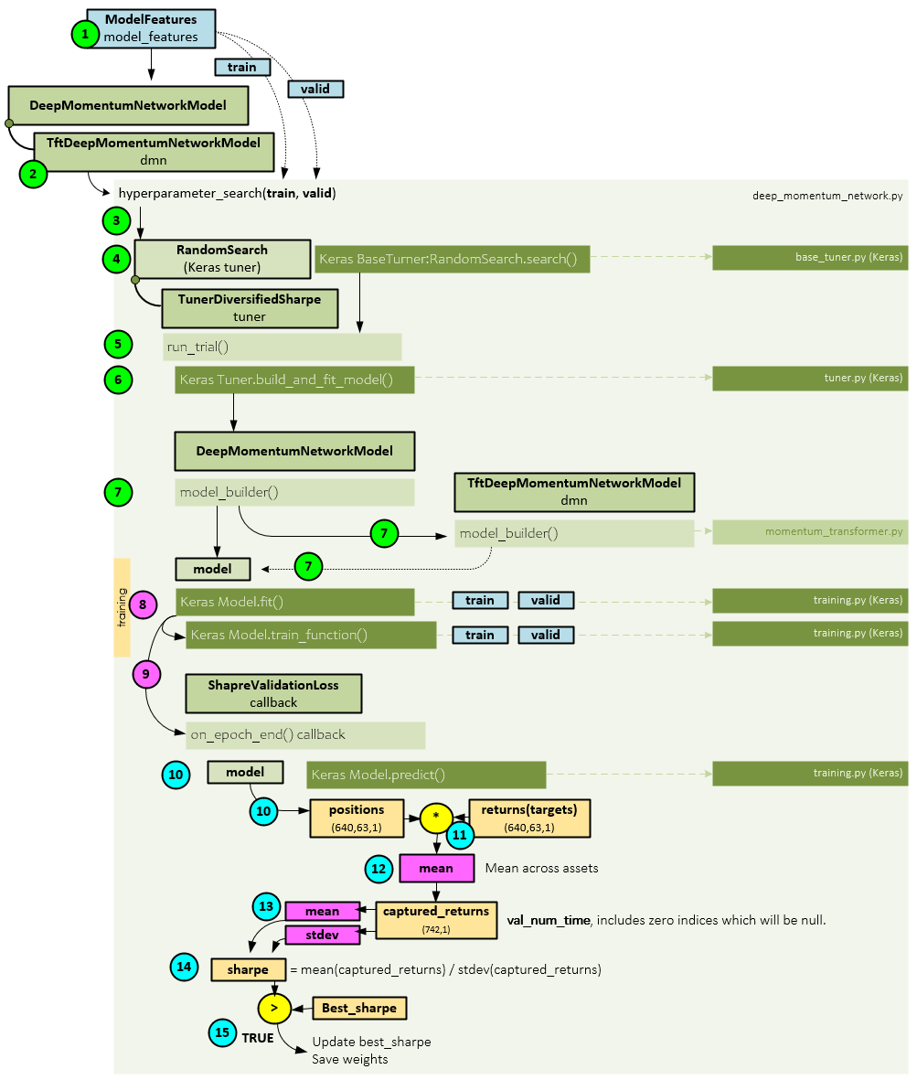
When training, the following steps occur.

The train and valid datasets are retrieved from the ModelFeatures and…
… sent to the TftDeepMomentumNetworkModel, which inherits from the real workhorse, the DeepMomentumNetworkModel.
All training occurs within the hyperparameter_search() function of the base class DeepMomentumNetworkModel. Using the TFT-SHORT configuration, which uses 63 steps and no change points, the optimal settings found were: hidden = 10, dropout = 0.1, max_grad = 0.01, learning_rate = 0.01 with a batch size = 256.
The TunerDiversifiedSharpe object, which is inherited from the Keras RansomSarch tuner is used to perform the hyper parameter search via the RandomSearch.search() function.
Inside the search() function, the TunerDiversifiedSharpe run_trial() method is called on each set of hyper parameters.
Within the run_trial method, the Keras build_and_fit_model() function is called to a.) build the model, and then b.) train the model.
Keras then calls its internal model_builder() function which calls the inherited model_builder function of the TftDeepMomentumNetworkModel. This is where the Temporal Fusion Transformer (TFT) model is built and returned as the model.
The model is then passed to the Keras fit() function along with the train and valid datasets which internally calls the Keras Model.train_function() to do the training.
Upon completion of each epoch, the on_epoch_end() callback is called passing into it the model, train, and valid datasets.
Within the SharpeValidationLoss callback, the Keras predict() function is called to calculate the predicted positions.
The predicted positions (position sizes) are multiplied by the target returns, …
… and a segment mean is taken of the result across the assets to produce the captured_returns.
A mean and standard deviation are taken on the captured_returns.
The Sharpe ratio [6] is calculated using the mean and standard deviation of the captured_returns.
If the calculated sharpe ratio is greater than the best_sharpe ratio, the best_sharpe ratio is updated and the model weights saved.

The training process continues for 300 epochs or exits early if the early stopping conditions are met.

Step 5 – Model Evaluation

There are two main parts to model evaluation: a.) doing the evaluation to get the results, and b.) calculating the captured returns from the results.

The following steps occur during the model evaluation part.

First, the valid dataset is collected using the ModelFeatures
Next, the TftDeepMomentumNetworkModel.evaluate() method is run passing to it the valid dataset and best model previously trained during the training step. The evaluate function is implemented by the DeepMomentumNetworkModel base class.
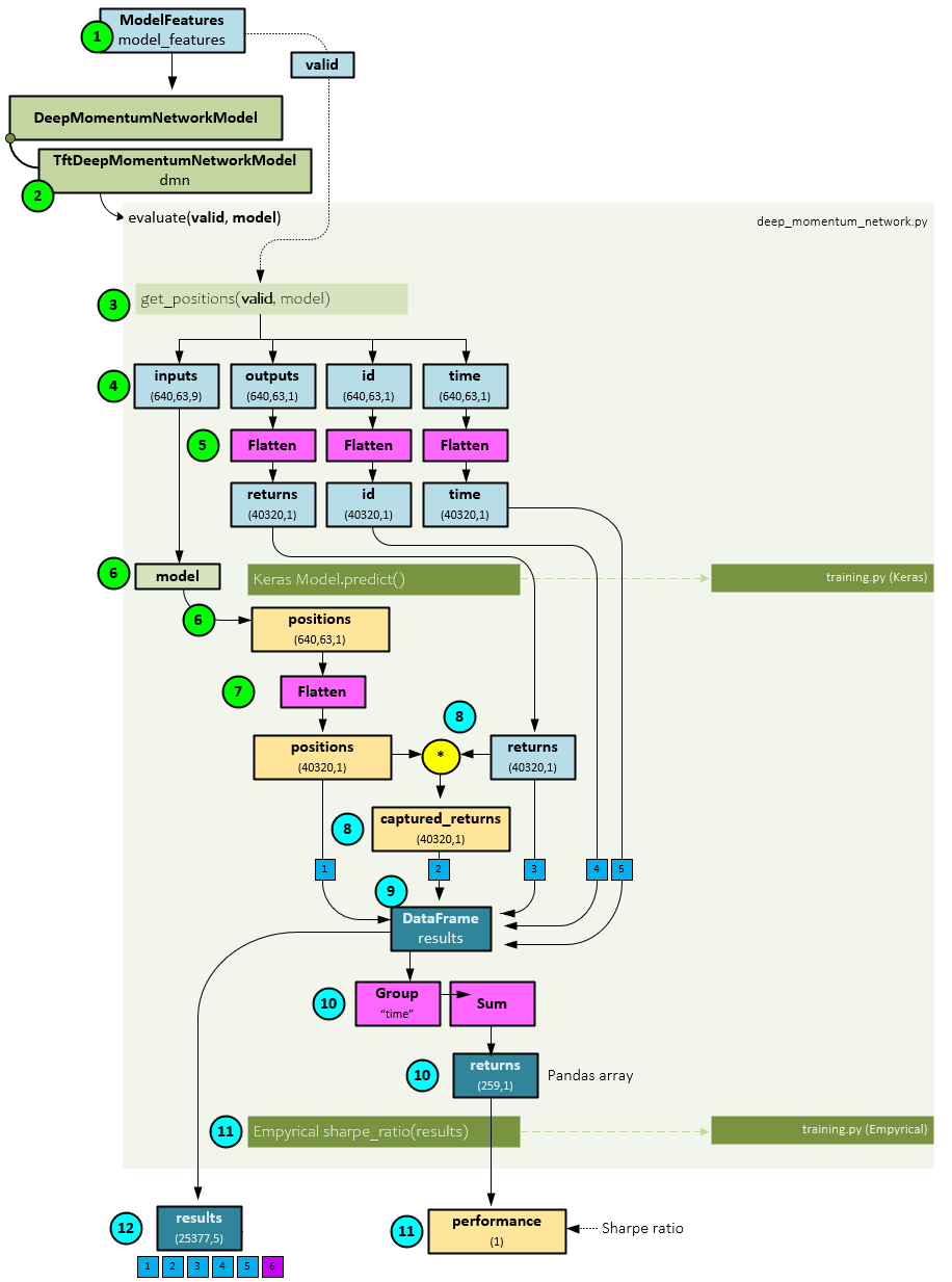
Within the evaluate function, the get_positions() function is called passing to it the valid dataset and best model.
Within the get_positions function, the inputs, outputs, id, and time sub-parts are extracted from the valid
Next, the outputs, id, and time are flattened across their first two axes so that all batched sequences are grouped together.
Next, the Keras predict() function is run on the model to calculate the positions which have a shape of (640,63,1).
The positions are flattened to match the shape of the inputs, outputs, id, and time.
Next, the positions are multiplied by the target returns to produce the captured returns.
The positions, captured returns, target returns, id, and time are added to a new DataFrame called results.
The DataFrame is grouped by time and summed across time for each asset to produce the returns Pandas array of shape (259,1).
A Sharpe ratio is calculated on the returns array using the sharpe_ratio() function to produce the performance value that is returned.
The results DataFrame is also returned.

Calculate Net Returns

Using the results DataFrame previously returned from the evaluate function, the net returns are calculated.

The following steps occur when calculating the net returns.

A main loop cycles through each ticker in the results DataFrame.
On each ticker, a Slice is made separating the results data from the current ticker into the slice(id) data slice with a shape (252,6) which contains the previous 5 items from the results (positions, captured returns, target returns, id, and time) with an added sixth element for daily volatility.
The daily volatility from the slice is multiplied by the square root of 252 to create the annualized_vol(atility).
Next, the position from the slice is multiplied by the VOL_TARGET of 0.15…
… and then divided by the annualized_vol to produce the scaled_position.
A Pandas diff and abs are taken of the scaled_position to produce the scaled_pos_diff.
The scaled_pos_diff is multiplied by a cost array containing six different cost settings for 0.5, 1.0, 1.5, 2.0, 2.5 and 3.0 basis points of cost, which produces the transaction_cost.
The transaction_cost is subtracted from the captured_returns from the slice to produce the
All net_captured_returns are Concat(enated) together to produce the full captured_returns, which is returned.

Step 6 – Model Inference

The model inferencing is basically the same as model evaluating with two main differences: a.) the inferencing is run on the test_sliding dataset and b.) a sliding window is used in the calculations.

The following steps occur when running the model inferencing with a sliding window.

First, the test_sliding dataset is collected using the ModelFeatures
Next, the TftDeepMomentumNetworkModel.evaluate() method is run passing to it the test_sliding dataset and best model previously trained during the training step. The DeepMomentumNetworkModel base class implements the evaluate
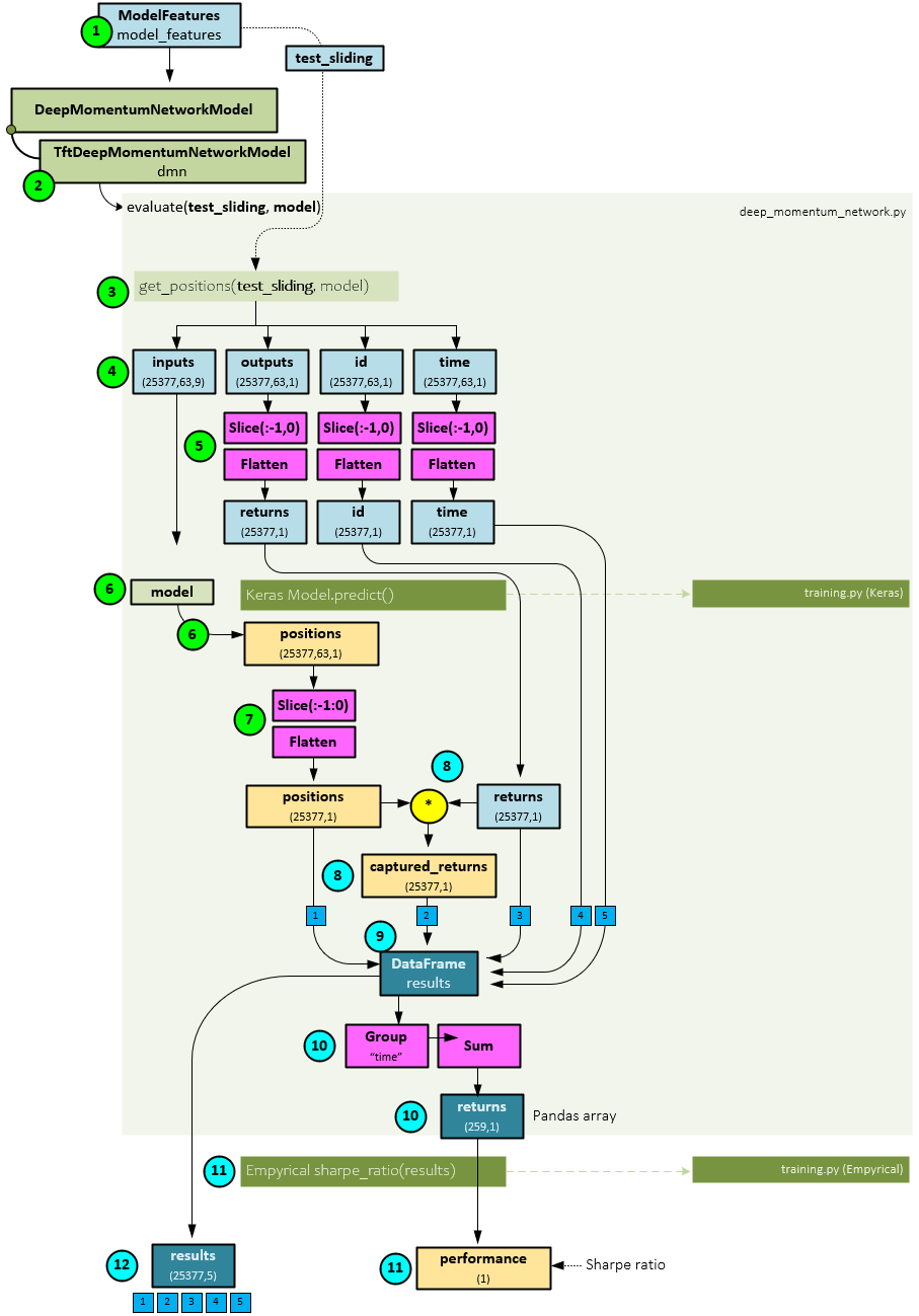
Within the evaluate function, the get_positions() function is called passing to it the test_sliding dataset and best model.
Within the get_positions() function, the inputs, outputs, id, and time sub-parts are extracted from the valid
Next, the outputs, id, and time are sliced, taking the last item of axis=1, then flattened across their first two axes so that all batched sequences are grouped together.
Next, the Keras predict() function is run on the model to calculate the positions which have a shape of (640,63,1).
The positions are sliced, taking the last item of axis=1, then flattened to match the shape of the inputs, outputs, id, and time.
Next, the positions are multiplied by the target returns to produce the captured returns.
The positions, captured returns, target returns, id, and time are added to a new DataFrame called results.
The DataFrame is grouped by time and summed across time for each asset to produce the returns Pandas array of shape (259,1).
A Sharpe ratio is calculated on the returns array using the Empyrical.sharpe_ratio() function to produce the performance value that is returned.
The results DataFrame is also returned.

The net returns are calculated using the same method as described above in part B of Step 5 – Model Evaluation.

Momentum Transformer Model Details

The Momentum Transformer uses a decoder only Temporal Fusion Transformer (TFT) model, which means it performs all the main steps of the TFT, except for the future variable processing. The SharpeRatioLoss layer is new to the Momentum Transformer and is used to optimize the model toward position sizes that have an increased Sharpe ratio. “The Sharpe ratio compares the return of an investment with its risk.” [6]

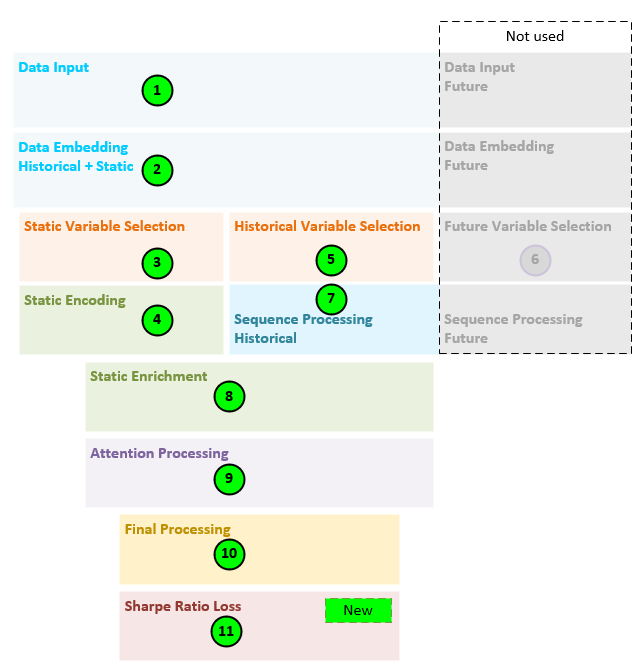
Momentum Transformer Model Overview (Decoder Only)

The general steps performed by the decoder only TFT model are as follows.

All data, comprising the ticker, and 8 other numerical values (norm daily return, norm monthly return, norm quarterly return, norm biannual return, norm annual return, macd(8,24), macd(16,48) and macd(32,96) are fed into the model.
The data inputs are transformed into a set of embeddings.
Static variable selection is performed on the static embedding (e.g., the ticker embedding).
Static encoding is performed to create the static enrichment, static variable selection inputs, and static state h and state c values.
Historical variable selection is performed on the remaining 8 numerical embeddings.
Given this is a decoder only TFT, nothing is done for step 6.
Next, the LSTM sequence processing is performed on the historical data only as this is a decoder only model.
Static enrichment is performed to enrich the data with the static values.
Attention processing occurs to learn more long-term relationships in the data.
Final processing produces the final position size predictions.
And a new Sharpe Loss layer is used to calculate the loss in such a way that maximizes the Sharpe ratio based on the position sizes predicted.

The following sections go through the details of each step outlined above.

Model: Data Input

Nine data streams are fed into the model where the first (ticker) is considered categorical and static, and all others are numerical and known.

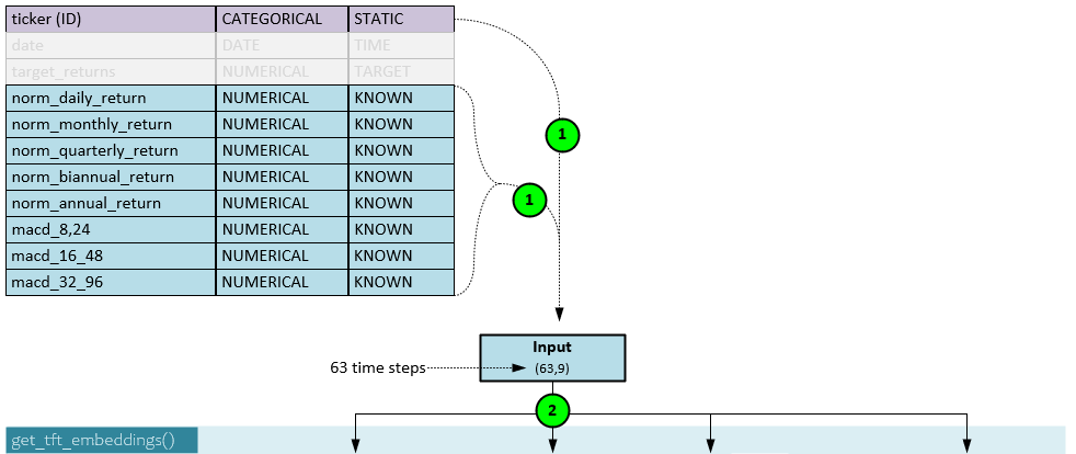
All input data streams (1) are loaded into the Input with a shape of 63 steps x 9 data streams. Note, the batch size is not shown but would otherwise be shown in the first axis such as (b,63,9).

Model: Embedding Transformation

All input data are transformed into embeddings using either an Embedding layer for categorical data or Dense linear layers for numerical data.

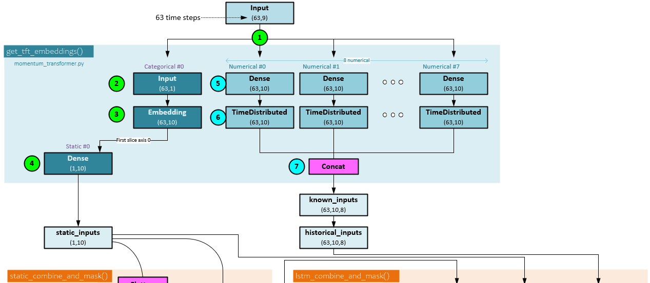
When transforming inputs to their respective embeddings, the following steps occur.

The Inputs are sent into the embedding processing with a shape of (b,63,9) indicating there are 9 data streams with 63 steps each.
The static data streams (of which there is only one for ‘ticker’) is sliced from the input, and …
… sent through the Embedding layer for the static data stream consists of categorical values (e.g., and index for each ticker). The Embedding has an output shape (b,63,10) as 10 hidden units are used.
The first temporal step in the embedding is sliced and sent to a Dense layer to produce the static_inputs with shape (1, 10).
Each numerical data stream of the Input is sent through its own individual Dense layer …
… followed by a TimeDistributed layer where each output is of shape (63,10) given the hidden size of 10.
All 8 numeric embeddings are concatenated together to produce the known_inputs of shape (63,10,8). The known_inputs are renamed the historical_inputs.

Model: Static Variable Selection

The static Variable Selection Network (VSN) helps weigh the importance of the static data stream given its impact on the predictions. Only one data stream (‘ticker’) ends up flowing through the static VSN.

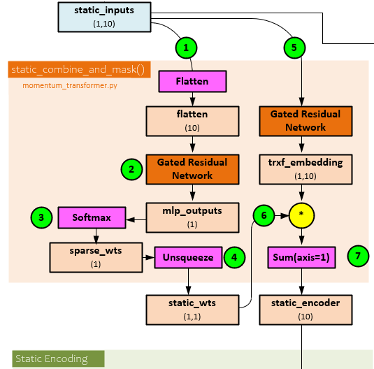
The following steps occur when processing the static Variable Selection Network.

The static_input is flattened to create the flatten tensor of shape (10).
The flatten tensor is sent through a Gated Residual Network (GRN) to produce the mlp_outputs of shape (1).
A Softmax is run on the mlp_outputs which does not do much given there is only one input data stream but produces the sparce_wts of shape (1).
An Unsqueeze operation expands the dimensions producing the static_wts of shape (1,1).
The static_inputs is sent unflattened through a second GRN to produce the trx_embedding of shape (1,10).
The static_wts are multiplied by the trx_embedding and …
… a Sum is run along axis=1 to produce the static_encoder output of shape (10).

Model: Static Encoding

Using the static_encoder output, the static encodings are created. These encodings are used for static enrichment, historical variable selection, and as the h and c states for the LSTM sequence processing.

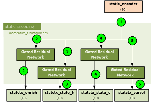
The following steps occur to create the static encodings.

The static_encoder of shape (10) is sent to the static encoding process and runs through four GRN
The first GRN processes the static_encoder to produce the statctx_enrich of shape (10) later used for static enrichment.
The second GRN processes the static_encoder to produce the statctx_state_h of shape (10) later used as the ‘h’ state for the LSTM during sequence processing.
The third GRN processes the static_encoder to produce the statctx_state_c of shape (10) later used as the ‘c’ state for the LSTM during sequence processing.
The fourth GRN processes the static_encoder to produce the statctx_varsel of shape (10) later used as input to the historical variable selection.

Model: Historical Variable Selection

The historical Variable Selection Network (VSN) helps weigh the importance of the historical data streams given their impact on the predictions. Eight data streams (‘norm daily return’, ‘norm monthly return’, ‘norm quarterly return’, ‘norm biannual return’, ‘norm annual return’, ‘macd(8,24)’, ‘macd(16,48)’ and ‘macd(32,96)’) flow through the historical VSN.

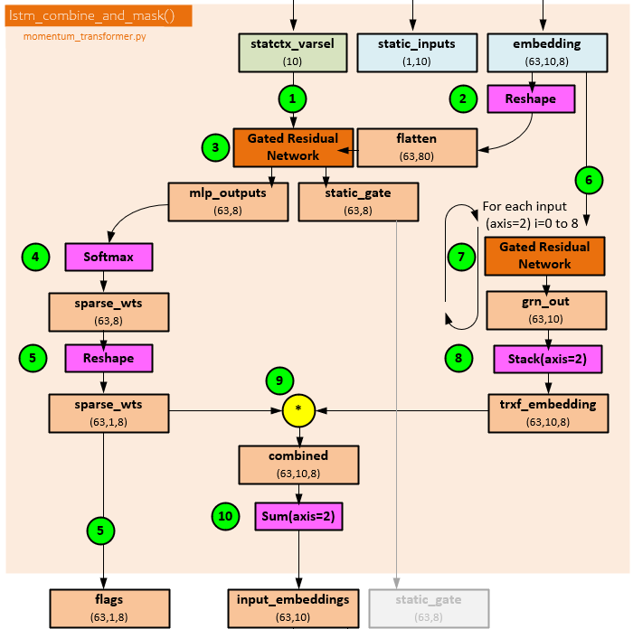
The following steps occur during historical variable selection.

The statctx_varsel of shape (10), previously calculated during static encoding, is sent …
… along with the previous historical_inputs of shape (63,10,8) now renamed embedding (63,10,8) that is reshaped to (63,80) …
… to a GRN that produces the mlp_outputs of shape (63,8) and static_gate of shape (63,8) that is not used.
A Softmax is run on the mlp_outputs to produce the sparse_wts of shape (63,8).
The sparse_wts are reshaped to a shape of (63,1,8) and are returned as the flags (63,1,8) output.
Each of the 8 data streams within the embedding (renamed historical_inputs) of shape (63,10,8) are processed individually.
Each individual slice of shape (63,10,8) is sent to a separate GRN to produce the grn_out(i) with shape (63,10).
All 8 grn_out outputs are Stacked together to produce the trxf_embedding of shape (63,10,8).
The trxf_embedding of shape (63,10,8) is multiplied by the sparse_wts of shape (63,1,8) to produce the combined of shape (63,10,8).
A Sum is taken of the combined (63,10,8) along the axis=2 to produce the input_embeddings of shape (63,10), which is returned.

Model: Sequence Processing

The sequence processing runs a single LSTM layer on the input_embedding returned by the historical variable selection previously discussed, while using the ‘h’ and ‘c’ states produced during the static encoding process.

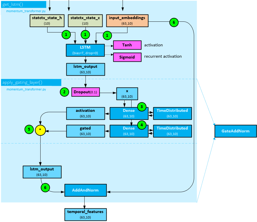
The following steps occur when processing the sequence on the decoder side.

The state ‘h’ and ‘c’ from the static embedding, and input_embeddings of shape (63,10) from the historical variable selection are sent to an LSTM layer which uses Tanh for the activation and Sigmoid for the recurrent activation to produce the lstm_output of shape (63,10).
The lstm_output of shape (63,10) is sent through a Droput layer with a dropout ratio of 0.1 to produce x with shape (63,10). Note, steps 2-5 occur within the apply_gating_layer() function in the py file.
A Dense layer followed by a TimeDistributed layer are run on x of shape (63,10) to produce the activation of shape (63,10.
Next, a second Dense layer followed by a TimeDistributed layer are run on the on x of shape (63,10) to produce the gated of shape (63,10).
The activation (63,10) and gated (63,10) are multiplied together to get the lstm_output of shape (63,10).
The lstm_output (63,10) and input_embedding (63,10) are run through an AddAndNorm layer which adds the two together and runs the result through a LayerNormalization layer to produce the temporal_features output of shape (63,10)

Note, steps 2-6 make up the processing within a GateAddNorm layer.

Model: Static Enrichment

Static enrichment involves applying the static enrichment, calculated during static encoding, to the temporal_features calculated during the sequence processing using a GRN.

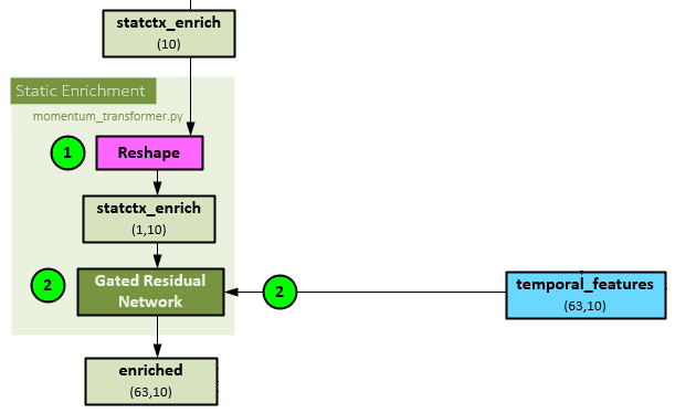
During static enrichment, the following steps take place.

The statctx_enrich of shape (10), previously calculated during static encoding is reshaped to a shape of (1,10).
Next, the temporal_features of shape (63,10), created during the sequence processing, and reshaped statctx_enrich are both run through a GRN layer to produce the enriched of shape (63,10)

Model: Attention Processing

Attention processing uses an InterpretableMultiHeadAttention layer to apply the Q, K, V self-attention algorithm [7] to the enriched data. Attention helps learn long term patterns within the temporal data.

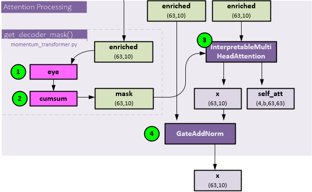
The following steps occur during the attention processing.

The enriched (63,10) data, previously created in the static enrichment step, is sent through the TensorFlow eye function, …
… and then TensorFlow cumsum function to create the mask of shape (63,10).
The enriched (63,10) is sent along with the mask (63,10) to the InterpretableMultiHeadAttention layer for attention processing which produces the x (63,10) and self_att (4,b,63,63) outputs. The self_att variable is helpful in visualizing where the attention is focused within the data which can provide helpful insights.

As a final step, the enriched (63,10) and x (63,10) attention output are run through a GateAddNorm layer to produce the final x output of shape (63,10).

Model: Final Processing

The final processing combines the x attention output with the temporal_features sequential processing output to produce the final output of predicted position sizes.

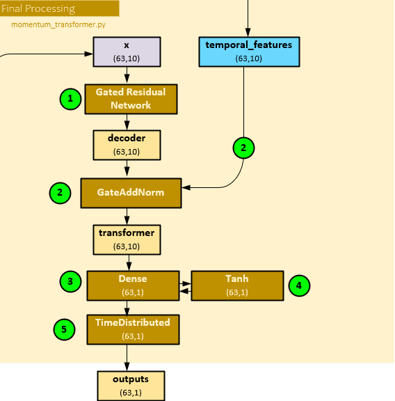
The following steps occur during the final process.

First the x (63,10) attention output is run through a GRN layer to produce the decoder (63,10) output.
Next, the decoder (63,10) and temporal_features (63,10) sequential processing output are combined with a GateAddNorm layer to produce the transformer output of shape (63,10).
The transformer (63,10) is run though a Dense linear layer, …
… followed by a Tanh activation function, …
… followed by a TimeDistributed layer to produce the final outputs of shape (63,1) which make up the position sizing predictions at each of the 63 steps.

Model: Loss Calculation

The SharpeLoss layer calculates the loss in such a way that maximizes the Sharpe ratio based on the position predictions produced during the final processing.

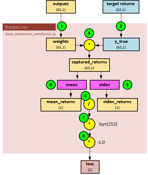
The following steps occur when calculating the loss for the model.

First the outputs (63,1) tensor, previously produced by the final processing which contains the position size predictions, is renamed to weights.
The target returns (63,1) tensor from the input data is renamed to y_true.
The weights (predicted position sizes) tensor is then multiplied by the y_true tensor (the target returns) to produce the captured_returns of size (63,1).
A mean is taken of the captured_returns to produce the mean_returns of size (1)
A stdev (standard deviation) is taken of the captured_returns to produce the stdev_returns of size (1).
The mean_returns (1) is divided by the stdev_returns (1), …
…, multiplied by the square root of 252 to annualize, …
… and multiplied by -1.0 so that the model optimizes to maximize the Sharpe ratio. The result is returned as the loss of shape (1).

Summary

In this post, we have shown how the Momentum Transformer works by describing the data it uses, how the data is loaded and used during training, evaluation, and inferencing. Next, we described how training, evaluation and inferencing work, including the method for which returns are calculated.

And finally, we described how the internals of the model work including the differences between the Temporal Fusion Transformer Model (Decoder Only) used by the Momentum Transformer and the original Temporal Fusion Transformer [5] that has both an encoder and decoder.

Happy Deep Learning with higher Sharpe ratios!

[1] Trading with the Momentum Transformer: An Intelligent and Interpretable Architecture, by Kieran Wood, Sven Giegerich, Stephen Roberts, and Stefan Zohren, 2021-2022, arXiv:2112.08534

[2] GitHub: kieranjwood/trading-momentum-transformer, by Kieran Wood, 2022, GitHub

[3] Returns to Buying Winners and Selling Losers: Implications for Stock Market Efficiency, by Narasimhan Jegadeesh and Sheridan Titman, 1993, SciSpace

[4] Portfolio rebalancing based on time series momentum and downside risk, by Xiaoshi Guo and Sarah M Ryan, 2021, Oxford Academic

[5] Temporal Fusion Transformers for Interpretable Multi-horizon Time Series Forecasting, by Bryan Lim, Sercan O. Arik, Nicolas Loeff, and Tomas Pfister, 2019-2020, arXiv:1912.09363

[6] Sharpe Ratio: Definition, Formula, and Examples, by Jason Fernando, 2023, Investopedia

[7] Attention Is All You Need, by Ashish Vaswani, Noam Shazeer, Niki Parmar, Jakob Uszkoreit, Llion Jones, Aidan N. Gomez, Lukasz Kaiser, and Illia Polosukhin, 2017-2023, arXiv:1912.09363