

In this post we describe a method of calculating change points using gaussian processes as described in the paper “Slow Momentum with Fast Reversion: A Trading Strategy Using Deep Learning and Changepoint Detection” by Wood et. al. [1], published in 2021. In addition, we show how the change point synthetic data enhances the Momentum Transformer model (see our previous post) as described in the paper, “Trading with the Momentum Transformer: An Intelligent and Interpretable Architecture” by Wood et. al. [2], published in 2022. The original code by Wood for change points and the Momentum Transformer analyzed can be found on GitHub at [3].
According to Wood et. al. [2], adding online change point detection can make the model “more robust to regime change[s]” such as market crashes and down-turns.
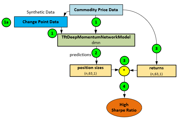
Change points are synthetic data created from the Commodity Price Data that show where the price data streams change from trending up to trending down and vice versa. In general, with change point data, the Momentum Transformer learns from both the Commodity Price Data (1) and the calculated change points (1a) to make position size predictions (2) that when combined with known returns (3) produce a high Sharpe ratio (4).
Because the Momentum Transformer is based on the Temporal Fusion Transformer [4], this model is ideal for synthetic data additions to the input data, such as change points. Change points define the locations in the data stream where meaningful changes occur in the mean, variance, and/or overall distribution of the data.
See our previous posts on “Understanding Adaptive LSTM-Autoencoder Change Point Detection” and “Understanding Contrastive Change Point Detection” for a few example methods of calculating change point synthetic data.
See our previous post “Understanding TFT Momentum Rebalancing for High Sharpe Ratios” to better understand how the Momentum Transformer model works.
Potential Results
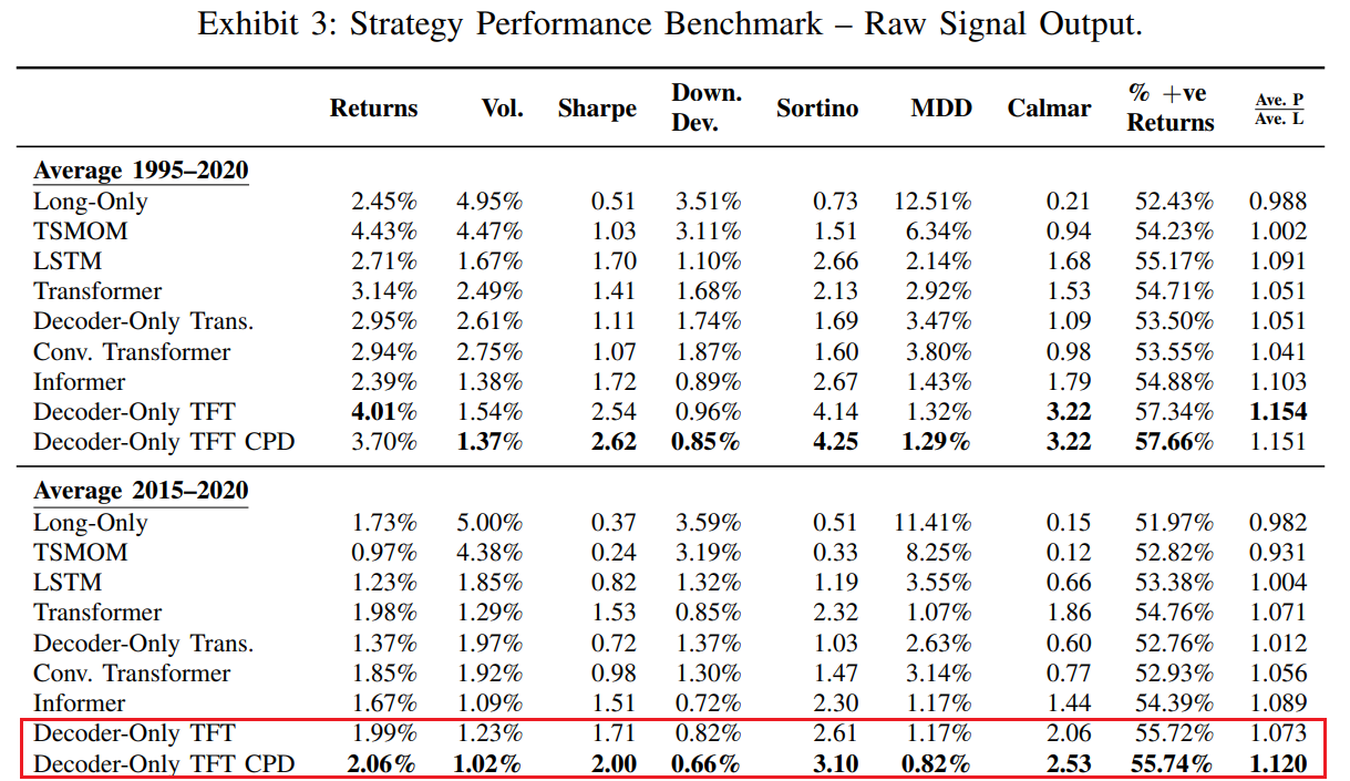
For the time period between 2015 to 2020, combining change points with the Momentum Transformer model increased the Sharpe ratio by 17%, from 1.71 to 2.0 on average results as shown by Wood et. al. [2].
Calculating Change Points
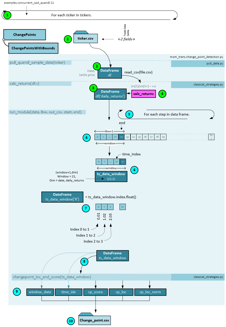
Change points are calculated by running the examples.concurrent_cpd_quandl.py script with the window size used to look for change points, such as 21 for a 21-period window. This script can be found on Wood’s GitHub at [3].
The following steps occur when calculating the change points for each ticker.
- Each ticker is processed in parallel on separate process.
- Within each process the change points for a single ticker are processed based on that ticker’s price data csv file located in the quandl folder, which is read into a DataFrame.
- Next, the calc_returns() function is run to create the DataFrame ‘daily_returns’ field of data.
- The calc_returns() function divides the previous value by the current in sequence and then subtracts 1.0 to calculate the returns.
- The input data stream of return values is processed in windows of data with as size of ‘window’ (e.g., a window = 21 for 21-periods). After processing each window, the data is stepped one step to the right in time to create the next data window for processing.
- Each window of data is placed into a new ts_data_window DataFrame, which has a shape of (22,2) with two items in the axis=1 dimensions: 1.) the daily returns, and 2.) the date. The ‘daily_returns’ field is renamed ‘Y’.
- A new data field is added to the ts_data_window DataFrame containing a float conversion of the start and end index of each field. For example, the first item is set to 0.01 for starting index 0 and ending index 1. The next item is set to 1.02 for starting index of 1 and ending index of 2, and so on. This new field is named ‘X’.
- The ts_data_window DataFrame is passed to the changepoint_loc_and_scores() function used to create the change points. This function is found in the py script.
- The changepoint_loc_and_scores() function (discussed later) returns the cp_score, cp_loc(ation), and cp_loc_norm for the normalized change point location.
- The window_date, time_idx, cp_score, cp_loc, cp_loc_norm values are then saved to the changepoint CSV for the ticker processed.
ChangePoint_Loc_And_Score Function
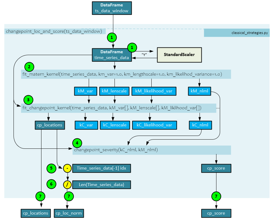
The changepoint_loc_and_score() function calculates the change point within each single window of data. For example, when a window size of 21 is used, the DataFrame contains 21+2, or 22 items. This function is in the classical_strategies.py script.
The following steps occur when detecting the change point locations and score with a data window.
- First the data window ts_data_window DataFrame is passed to the function and the ‘Y’ channel of data is normalized using a StandardScalar which centers and scales the data to the unit variance. The ts_data_window is renamed time_series_data.
- The scaled time_series_data is then passed to the fit_matern_kernel() function (discussed later) used to calculate the kernel parameters kM_var(iance), kM_lenscale, kM_likelihood_var(iance) as well as the kM_nlmn negative log marginal likelihood.
- Next the kM parameters are sent to the fit_changepoint_kernel() function along with the time_series_data. This function returns the cp_locations, kC_var(iance), kC_lenscale, kC_likelihood_var(iance), and kC_nlml negative log marginal likelihood.
- The kC_nlml from step #3 and kM_nlml from step #2 are sent to the changepoint_severity() function (discussed later) which calculates the cp_score.
- Next, the last index of the time_series_data is subtracted from the cp_locations, …
- … and the result is divided by the length of the time_series_data to produce the normalized cp_loc_norm value.
- The cp_locations, cp_loc_norm, and cp_score values are returned.
Fit_Matern_Kernel Function
The fit_matern_kernel() function fits the Matern kernel to the find the optimal parameters kM_var(iance), kM_lenscale, and kM_likelihood_var(iance) values and calculate the negative log marginal likelihood.
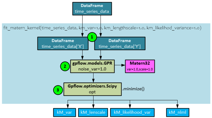
The following steps occur within the fit_matern_kernel() function.
- The X and Y data streams are extracted from the time_series_data DataFrame.
- The GPFlow GPR model is created with a Matern32 kernel and sent both the X and Y data streams.
- The GPFlow Scipy optimizer is run to find the minimized solution. Upon completion, the optimal parameters kM_var, kM_lenscale, and kM_likelihood_var are returned along with the negative log marginal likelihood kM_nlml value.
Fit_ChangePoint_Kernel Function
The fit_changepoint_kernel() function calculates the changepoint locations as well as the kC_nlml negative log marginal likelihood later used to help calculate the change point score.
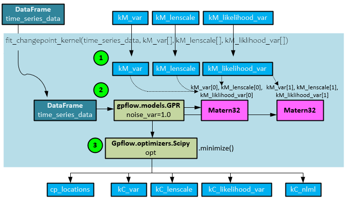
The following steps occur when calculating the cp_locations, kC parameters and kC_nlml negative log marginal likelihood value.
- The kM_var, kM_lenscale, kM_likelihood_var parameters, previously calculated by the fit_matern_kernel() function, are sent to this function.
- A GPFlow GPR model is created with two Matern32 kernels where the first is initialized with the first of the two sets of parameters and the second is initialized with the second set of parameters.
- The GPFlow Scipy optimizer is run to find the minimized solution. Upon completion, the optimal parameters kC_var, kC_lenscale, and kC_likelihood_var are returned along with the negative log marginal likelihood kC_nlml.
ChangePoint_Serverity Function
The changepoint_severity() function calculates the final cp_score value using the two previously calculated negative log marginal likelihood values kM_nlml and kM_nlml.
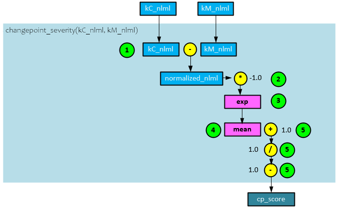
The following steps take place to calculate the cp_score value.
- The kM_nlml negative log marginal likelihood from the fit_matern_kernel() function is subtracted from the kC_nlml negative log marginal likelihood from the fit_changepoint_kernel() function to produce the normalized_nlml value, …
- … which is multiplied by -1.0, …
- … then run through an exp function, …
- … and a mean is taken of the result.
- A value of 1.0 is subtracted from 1.0 divided by the mean of step #4 above to produce the cp_score value which is returned.
Adding Change Points to the Momentum Transformer
Change point data is synthetic data that enhances the Momentum Transformer predictions. Each of the following sections describe the updates made to the Momentum Transformer to support change point data.
Before continuing, it is recommended that you read the previous post “Understanding TFT Momentum Rebalancing for High Sharpe Ratios” as the following sections build upon that discussion.
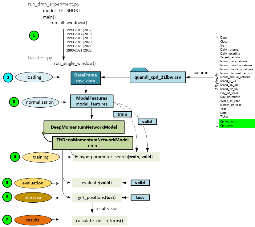
Overall Process with Change Point Synthetic Data
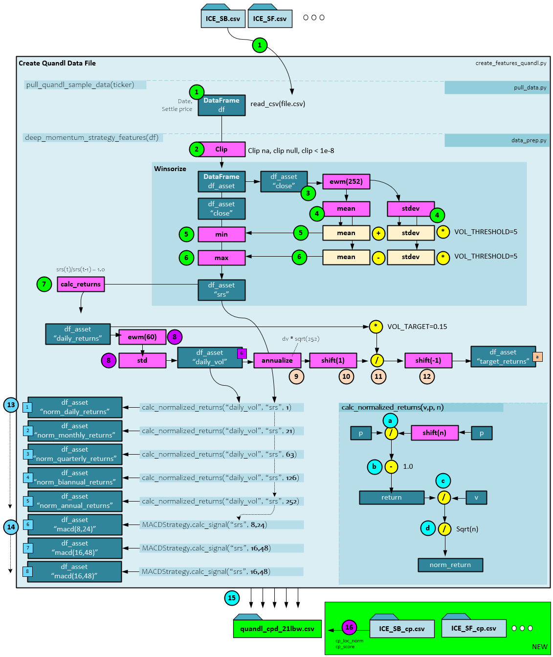
Adding the change point synthetic data does not change the overall process, but instead just adds two new input fields of data to the quandl_cpd_21lbw.csv file for a total of 23 fields now loaded into the DataFrame instead of 21. This occurs during step #2 below, where all other steps remain unchanged. Our previous post describes all other steps in detail.
Data Preparation with Change Points
The data preparation process only has a very small change when adding change point synthetic data – all steps are the same except for the last step #16 at the very end where the previously calculated change point data for each symbol is merged into the resulting quandl_cpd_21lbw.csv file. See our previous post for a full description of the data preparation process.
Data Input with Change Point Data
Loading data into the model also has only a small number of changes when adding the new synthetic change point data. The change point data adds two new fields loaded into the Input tensor.
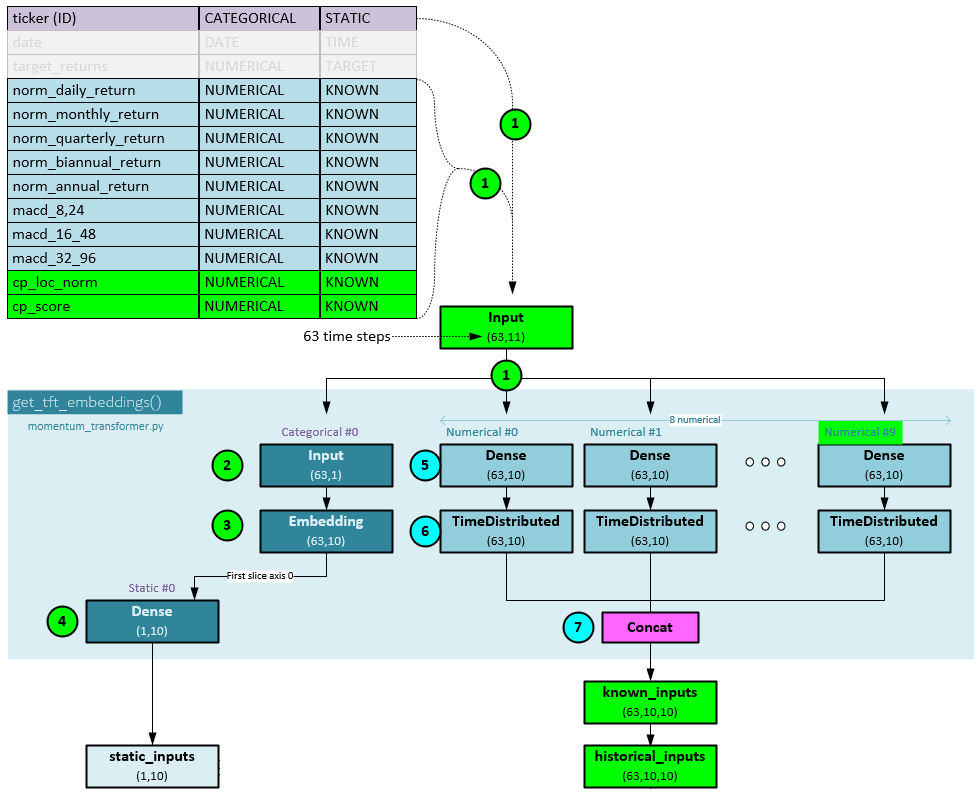
The data is loaded as before (1), but now two new fields are loaded; one for the cp_loc_norm (normalized change point location) and another for the cp_score (change point score). The Input tensor now has a shape of (63,11) instead of the original shape (63,9) used with no change point data. Steps 2-4 remain unchanged. In steps 5 and 6 two additional Dense and TimeDistributed layers are used to encode the newly added cp_loc_norm and cp_score values. In step 7, the 10 outputs (2 additional) are concatenated into the known_inputs which now has a shape of (63,10,10) for 63 steps, hidden size of 10, and 10 values that include the new cp_loc_norm and cp_score values.
See our previous post for details on the steps that follow which are unchanged with the new change point data.
Summary
In this post, we have shown how the Momentum Transformer works with change points by describing the how change points alter the overall process and data preparation stage. Next, we described how the change point data is loaded into the model.
And finally, we described how the change point data is calculated using a gaussian process method.
Happy Deep Learning Momentum Transformer and Change Points to get higher Sharpe ratios!
[1] Slow Momentum with Fast Reversion: A Trading Strategy Using Deep Learning and Changepoint Detection, by Kieran Wood, Stephen Roberts, and Stefan Zohren, 2021, arXiv:2105.13727
[2] Trading with the Momentum Transformer: An Intelligent and Interpretable Architecture, by Kieran Wood, Sven Giegerich, Stephen Roberts, and Stefan Zohren, 2021-2022, arXiv:2112.08534
[3] GitHub: kieranjwood/trading-momentum-transformer, by Kieran Wood, 2022, GitHub
[4] Temporal Fusion Transformers for Interpretable Multi-horizon Time Series Forecasting, by Bryan Lim, Sercan O. Arik, Nicolas Loeff, and Tomas Pfister, 2019-2020, arXiv:1912.09363