

In this blog post, we compare the Liquid closed-form continuous-time neural network (CfC), as described by [1], [2] and [3], to the Long-Short Term Memory (LSTM) neural network and a simple Linear neural network to see how each model learns to track a simple Sine curve over time.
To keep things simple, each test uses the same number of 82 inputs and have a single output which is trained to follow the Sine curve. The same AdamW optimizer is used with each model and the train/run cycle consists of a single batch for each cycle.
The train/run cycle used looks as follows.
- Use the past 82 points from the current position on the Sine curve as the current input.
- Run a forward pass with batch size = 1
- Run a backward pass with batch size = 1
- Step and apply the weight updates with the optimizer.
- And apply the weight updates and repeat.
- Move to the next position on the curve and repeat step #1 above.
Simple Linear Model
In our first test, we ran a simple Linear neural network with the following model.
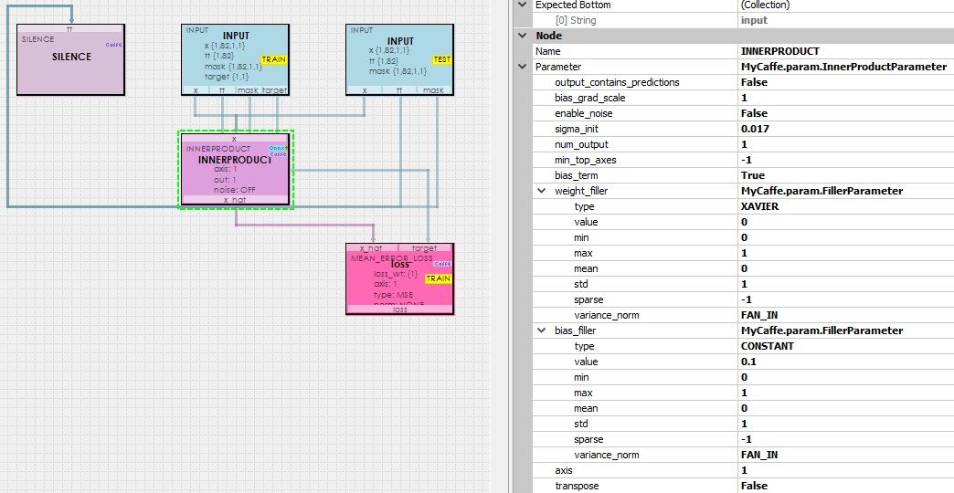
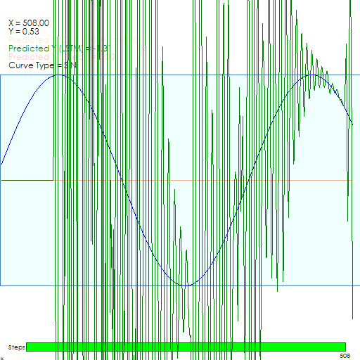
The Simple Linear model uses an InnerProduct layer which is sent the past 82 points on the Sine curve via the input blob x, the blobs tt and mask are ignored, and the target is set to the last of the 82 points for we want to learn to track the Sine curve.
To learn more about configuring the InnerProduct layer, see the InnerProductParameter.
When running, the model initially servos into the Sine curve after around 150 steps which is great!
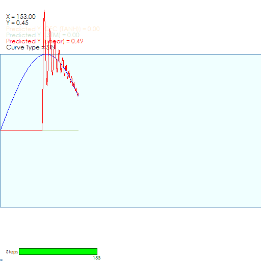
However, shortly after around 200 steps the predictions start experiencing significant jitter.
LSTM and Linear Model
Next, we added a Long-Short Term Memory (LSTM) layer to the model to learn the temporal nature of the Sine curve.
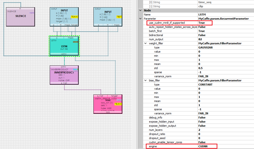
The LSTM + Linear model adds an LSTM layer to the InnerProduct layer which has a single output for the prediction, like the Simple Linear model. In addition, the NVIDIA CuDnn implementation is used for the low-level LSTM implementation because of its fast computation speed. The LSTM layer is configured to use 2 layers internally.
To learn more about configuring the LSTM layer, see the RecurrentParameter.
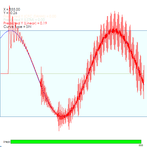
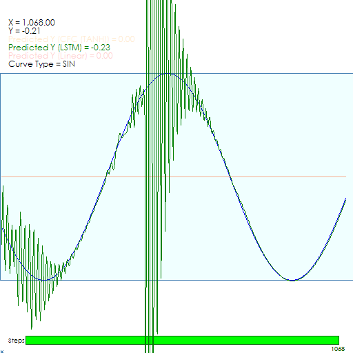
First the LSTM Model starts with a considerable amount of noise.
However, after around 900 iterations, the model learns to lock onto the Sine curve.
Liquid Closed-form continuous-time (CfC) Model
And finally, lets see how the Liquid Closed-form continuous-time (CfC) model performs when learning the Sine curve.
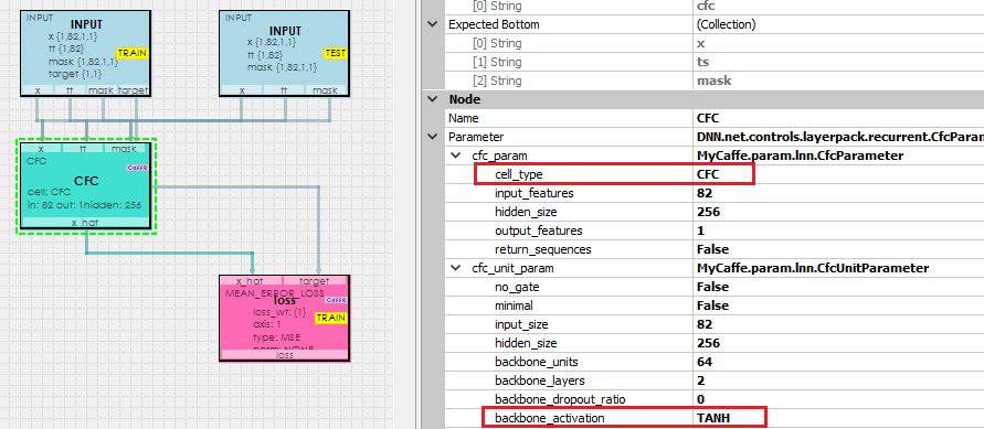
The CfC Model comprises a CfC Layer which internally uses the CfC Unit layer configured to use the TanH backbone activation with 2 internal backbone layers.
To learn more about configuring the CfC Layer see the CfCParameter.
To learn more about configuring the CfC Unit layer, see the CfCUnitParameter.
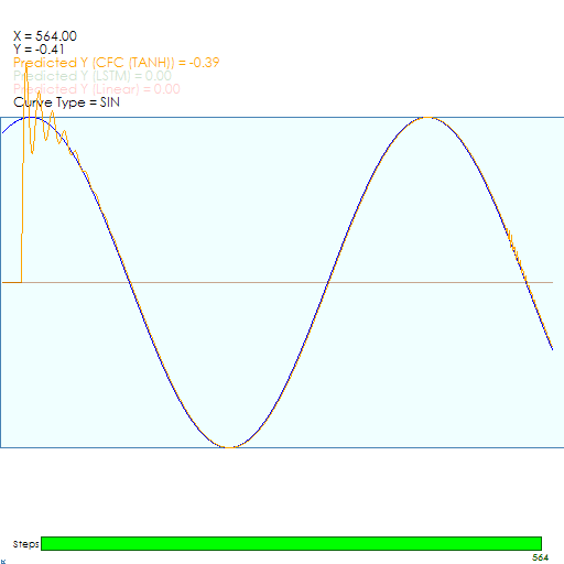
The CfC Model locks onto the target Sine curve very quickly in around 126 steps.
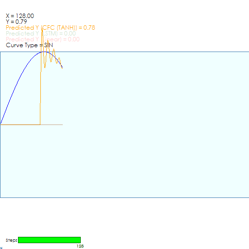
And once locked on the CfC model does a good job of staying on target, which is one of the benefits of the CfC model.
We believe this quick locking onto the target can be attributed to the servoing action caused by the combination of the internal Sigmoid function and inverse Sigmoid function that are combined within the CfC Unit Layer. To read more about how this works, see our blog post Closed-form Continuous-time Liquid Neural Net Models – A Programmer’s Perspective.
Comparison Summary
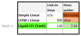
When comparing the Liquid CfC Model to the LSTM and Simple Linear models, there really is no comparison as the CfC locks on target over 7x faster than the LSTM and the Simple Linear is too noisy to be usable.
As a side note, we have observed the CfC Model experience a very small amount of jitter (as can be seen on the right side of the CfC image above) during very short durations which may be caused by a vanishing gradient. However, combining the LSTM with the CfC may eliminate this jitter as doing so is recommended by the original paper to alleviate the vanishing gradient problem [1], [2].
To dig into the source code for this post, see the TestTrainRealTimeComboNet function on the MyCaffe GitHub site.
Happy Deep Learning with MyCaffe and Liquid CfC Neural Networks!
[1] Closed-form Continuous-time Neural Models, by Ramin Hasani, Mathias Lechner, Alexander Amini, Lucas Liebenwein, Aaron Ray, Max Tschaikowski, Gerald Teschl, Daniela Rus, 2021, arXiv:2106.13898
[2] Closed-form continuous-time neural networks, by Ramin Hasani, Mathias Lechner, Alexander Amini, Lucas Liebenwein, Aaron Ray, Max Tschaikowski, Gerald Teschl, Daniela Rus, 2022, nature machine intelligence
[3] GitHub: Closed-form Continuous-time Models, by Ramin Hasani, 2021, GitHub